TensorFlow.js is a new version of the popular open-source library which brings deep learning to JavaScript. Developers can now define, train, and run machine learning models using the high-level library API.
Having started as a front-end library for web browsers, recent updates added experimental support for Node.js. This allows TensorFlow.js to be used in backend JavaScript applications without having to use Python.
Reading about the library, I wanted to test it out with a simple task… 🧐
Use TensorFlow.js to perform visual recognition on images using JavaScript from Node.js
Unfortunately, most of the documentation and example code provided uses the library in a browser. Project utilities provided to simplify loading and using pre-trained models have not yet been extended with Node.js support. Getting this working did end up with me spending a lot of time reading the Typescript source files for the library. 👎
However, after a few days’ hacking, I managed to get this completed! Hurrah! 🤩
Before we dive into the code, let’s start with an overview of the different TensorFlow libraries.
TensorFlow
TensorFlow is an open-source software library for machine learning applications. TensorFlow can be used to implement neural networks and other deep learning algorithms.
Released by Google in November 2015, TensorFlow was originally a Python library. It used either CPU or GPU-based computation for training and evaluating machine learning models. The library was initially designed to run on high-performance servers with expensive GPUs.
Recent updates have extended the software to run in resource-constrained environments like mobile devices and web browsers.
TensorFlow Lite
Tensorflow Lite, a lightweight version of the library for mobile and embedded devices, was released in May 2017. This was accompanied by a new series of pre-trained deep learning models for vision recognition tasks, called MobileNet. MobileNet models were designed to work efficiently in resource-constrained environments like mobile devices.
TensorFlow.js
Following Tensorflow Lite, TensorFlow.js was announced in March 2018. This version of the library was designed to run in the browser, building on an earlier project called deeplearn.js. WebGL provides GPU access to the library. Developers use a JavaScript API to train, load and run models.
TensorFlow.js was recently extended to run on Node.js, using an extension library called tfjs-node.
The Node.js extension is an alpha release and still under active development.
Importing Existing Models Into TensorFlow.js
Existing TensorFlow and Keras models can be executed using the TensorFlow.js library. Models need converting to a new format using this tool before execution. Pre-trained and converted models for image classification, pose detection and k-nearest neighbours are available on Github.
Using TensorFlow.js in Node.js
Installing TensorFlow Libraries
TensorFlow.js can be installed from the NPM registry.
Both Node.js extensions use native dependencies which will be compiled on demand.
Loading TensorFlow Libraries
TensorFlow’s JavaScript API is exposed from the core library. Extension modules to enable Node.js support do not expose additional APIs.
12345
consttf=require('@tensorflow/tfjs')// Load the binding (CPU computation)require('@tensorflow/tfjs-node')// Or load the binding (GPU computation)require('@tensorflow/tfjs-node-gpu')
Looking at the source code, the mobilenet library is a wrapper around the underlying tf.Model class. When the load() method is called, it automatically downloads the correct model files from an external HTTP address and instantiates the TensorFlow model.
The Node.js extension does not yet support HTTP requests to dynamically retrieve models. Instead, models must be manually loaded from the filesystem.
After reading the source code for the library, I managed to create a work-around…
Loading Models From a Filesystem
Rather than calling the module’s load method, if the MobileNet class is created manually, the auto-generated path variable which contains the HTTP address of the model can be overwritten with a local filesystem path. Having done this, calling the load method on the class instance will trigger the filesystem loader class, rather than trying to use the browser-based HTTP loader.
Models for TensorFlow.js consist of two file types, a model configuration file stored in JSON and model weights in a binary format. Model weights are often sharded into multiple files for better caching by browsers.
Looking at the automatic loading code for MobileNet models, models configuration and weight shards are retrieved from a public storage bucket at this address.
The template parameters in the URL refer to the model versions listed here. Classification accuracy results for each version are also shown on that page.
According to the source code, only MobileNet v1 models can be loaded using the tensorflow-models/mobilenet library.
The HTTP retrieval code loads the model.json file from this location and then recursively fetches all referenced model weights shards. These files are in the format groupX-shard1of1.
Downloading Models Manually
Saving all model files to a filesystem can be achieved by retrieving the model configuration file, parsing out the referenced weight files and downloading each weight file manually.
I want to use the MobileNet V1 Module with 1.0 alpha value and image size of 224 pixels. This gives me the following URL for the model configuration file.
This example code is provided by TensorFlow.js to demonstrate returning classifications for an image.
1234
constimg=document.getElementById('img');// Classify the image.constpredictions=awaitmodel.classify(img);
This does not work on Node.js due to the lack of a DOM.
The classifymethod accepts numerous DOM elements (canvas, video, image) and will automatically retrieve and convert image bytes from these elements into a tf.Tensor3D class which is used as the input to the model. Alternatively, the tf.Tensor3D input can be passed directly.
Rather than trying to use an external package to simulate a DOM element in Node.js, I found it easier to construct the tf.Tensor3D manually.
Generating Tensor3D from an Image
Reading the source code for the method used to turn DOM elements into Tensor3D classes, the following input parameters are used to generate the Tensor3D class.
1234
constvalues=newInt32Array(image.height*image.width*numChannels);// fill pixels with pixel channel bytes from imageconstoutShape=[image.height,image.width,numChannels];constinput=tf.tensor3d(values,outShape,'int32');
pixels is a 2D array of type (Int32Array) which contains a sequential list of channel values for each pixel. numChannels is the number of channel values per pixel.
Creating Input Values For JPEGs
The jpeg-js library is a pure javascript JPEG encoder and decoder for Node.js. Using this library the RGB values for each pixel can be extracted.
1
constpixels=jpeg.decode(buffer,true);
This will return a Uint8Array with four channel values (RGBA) for each pixel (width * height). The MobileNet model only uses the three colour channels (RGB) for classification, ignoring the alpha channel. This code converts the four channel array into the correct three channel version.
The MobileNet model being used classifies images of width and height 224 pixels. Input tensors must contain float values, between -1 and 1, for each of the three channels pixel values.
Input values for images of different dimensions needs to be re-sized before classification. Additionally, pixels values from the JPEG decoder are in the range 0 - 255, rather than -1 to 1. These values also need converting prior to classification.
TensorFlow.js has library methods to make this process easier but, fortunately for us, the tfjs-models/mobilenet library automatically handles this issue! 👍
Developers can pass in Tensor3D inputs of type int32 and different dimensions to the classify method and it converts the input to the correct format prior to classification. Which means there’s nothing to do… Super 🕺🕺🕺.
Obtaining Predictions
MobileNet models in Tensorflow are trained to recognise entities from the top 1000 classes in the ImageNet dataset. The models output the probabilities that each of those entities is in the image being classified.
The full list of trained classes for the model being used can be found in this file.
The tfjs-models/mobilenet library exposes a classify method on the MobileNet class to return the top X classes with highest probabilities from an image input.
Having worked how to use the TensorFlow.js library and MobileNet models on Node.js, this script will classify an image given as a command-line argument.
source code
Save this script file and package descriptor to local files.
testing it out
Download the model files to a mobilenet directory using the instructions above.
Install the project dependencies using NPM
1
npminstall
Download a sample JPEG file to classify
1
wgethttp://bit.ly/2JYSal9 -O panda.jpg
Run the script with the model file and input image as arguments.
1
nodescript.jsmobilenet/model.jsonpanda.jpg
If everything worked, the following output should be printed to the console.
1234
classificationresults:[{className:'giant panda, panda, panda bear, coon bear',probability:0.9993536472320557}]
The image is correctly classified as containing a Panda with 99.93% probability! 🐼🐼🐼
Conclusion
TensorFlow.js brings the power of deep learning to JavaScript developers. Using pre-trained models with the TensorFlow.js library makes it simple to extend JavaScript applications with complex machine learning tasks with minimal effort and code.
Having been released as a browser-based library, TensorFlow.js has now been extended to work on Node.js, although not all of the tools and utilities support the new runtime. With a few days’ hacking, I was able to use the library with the MobileNet models for visual recognition on images from a local file.
Getting this working in the Node.js runtime means I now move on to my next idea… making this run inside a serverless function! Come back soon to read about my next adventure with TensorFlow.js. 👋
Following all the events from the World Cup can be hard. So many matches, so many goals. Rather than manually refreshing BBC Football to check the scores, I decided to created a Twitter bot that would automatically tweet out each goal.
The Twitter bot runs on IBM Cloud Functions. It is called once a minute to check for new goals, using the alarm trigger feed. If new goals have been scored, it calls another action to send the tweet messages.
⚽️ GOAL ⚽️ 👨 Harry MAGUIRE (🏴 ) @ 30'. 👨 🏟 Sweden 🇸🇪 (0) v England 🏴 (1) 🏟#WorldCup
Once it was running, I need to ensure it was working correctly for the duration of the tournament. Using the IBM Cloud Logging service, I built a custom monitoring dashboard to help to me recognise and diagnose issues.
The dashboard showed counts for successful and failed activations, when they occurred and a list of failed activations. If issues have occurred, I can retrieve the failed activation identifiers and investigate further.
Let’s walk through the steps used to create this dashboard to help you create custom visualisations for serverless applications running on IBM Cloud Functions…
IBM Cloud Logging
IBM Cloud Logging can be accessed using the link on the IBM Cloud Functions dashboard. This will open the logging service for the current organisation and space.
All activation records and application logs are automatically forwarded to the logging service by IBM Cloud Functions.
Log Message Fields
Activation records and application log messages have a number of common record fields.
activationId_str - activation identifier for log message.
timestamp - log draining time.
@timestamp - message ingestion time.
action_str - fully qualified action name
Log records for different message types are identified using the type field. This is either activation_record or user_logs for IBM Cloud Functions records.
Activation records have the following custom fields.
duration_int - activation duration in milliseconds
status_str - activation status response (non-zero for errors)
message - activation response returned from action
time_date - activation record start time
end_date - activation record end time
Applications log lines, written to stdout or stderr, are forwarded as individual records. One application log line per record. Log message records have the following custom fields.
message - single application log line output
stream_str - log message source, either stdout or stderr
time_date - timestamp parsed from application log line
Finding Log Messages For One Activation
Use this query string in the ”Discover” tab to retrieve all logs messages from a particular activation.
This is the monitoring dashboard I created. It contains visualisations showing counts for successful and failed activations, histograms of when they occurred and a list of the recent failed activation identifiers.
It allows me to quickly review the previous 24 hours activations for issues. If there are notable issues, I can retrieve the failed activation identifiers and investigate further.
Before being able to create the dashboard, I needed to define two resources: saved searches and visualisations.
Saved Searches
Kibana supports saving and referring to search queries from visualisations using explicit names.
Using saved searches with visualisations, rather than explicit queries, removes the need to manually update visualisations’ configuration when queries change.
This dashboard uses two custom queries in visualisations. Queries are needed to find activation records from both successful and failed invocations.
Create a new “Saved Search” named “activation records (success)” using the following search query.
1
type: activation_record AND status_str: 0
Create a new “Saved Search” named “activation records (failed)” using the following search query.
1
type: activation_record AND NOT status_str: 0
The status_str field is set to a non-zero value for failures. Using the type field ensures log messages from other sources are excluded from the results.
Indexed Fields
Before referencing log record fields in visualisations, those fields need to be indexed correctly. Use these instructions to verify activation records fields are available.
Check IBM Cloud Functions logs are available in IBM Cloud Logging using the ”Discover” tab.
Click the “⚙️ (Management)” menu item on the left-hand drop-down menu in IBM Cloud Logging.
Click the ”Index Patterns” link.
Click the 🔄 button to refresh the field list.
Visualisations
Three types of visualisation are used on the monitoring dashboard. Metric displays are used for the activation counts, vertical bar charts for the activation times and a data table to list failed activations.
Visualisations can be created by opening the “Visualize” menu item and select a new visualisation type under the “Create New Visualization” menu.
Create five different visualisations, using the instructions below, before moving on to create the dashboard.
Activation Counts
Counts for successful and failed activations are displayed as singular metric values.
Select the “Metric” visualisation from the visualisation type list.
Use the “activation records (success)” saved search as the data source.
Ensure the Metric Aggregation is set to “Count”
Set the “Font Size” under the Options menu to 120pt.
Save the visualisation as “Activation Counts (Success)”
Repeat this process to create the failed activation count visualisation.
Use the “activation records (failed)” saved search as the data source.
Save the visualisation as “Activation Counts (Failed)”.
Activation Times
Activation counts over time, for successful and failed invocations, are displayed in vertical bar charts.
Select the “Vertical bar chart” visualisation from the visualisation type list.
Use the “activation records (success)” saved search as the data source.
Set the “Custom Label” to Invocations
Add an “X-Axis” bucket type under the Buckets section.
Choose “Date Histogram” for the aggregation, “@timestamp” for the field and “Minute” for the interval.
Save the visualisation as “Activation Times (Success)”
Repeat this process to create the failed activation times visualisation.
Use the “activation records (failed)” saved search as the data source.
Save the visualisation as “Activation Times (Failed)”
Failed Activations List
Activation identifiers for failed invocations are shown using a data table.
Select the “Data table” visualisation from the visualisation type list.
Use the “activation records (failed)” saved search as the data source.
Add a “Split Rows” bucket type under the Buckets section.
Choose “Date Histogram” for the aggregation, “@timestamp” for the field and “Second” for the interval.
Add a “sub-bucket” with the “Split Rows” type.
Set sub aggregation to “Terms”, field to “activationId_str” and order by “Term”.
Save the visualisation as “Errors Table”
Creating the dashboard
Having created the individual visualisations components, the monitoring dashboard can be constructed.
Click the “Dashboard” menu item from the left-and menu panel.
Click the “Add” button to import visualisations into the current dashboard.
Add each of the five visualisations created above.
Hovering the mouse cursor over visualisations will reveal icons for moving and re-sizing.
Re-order the visualisations into the following rows:
Activations Metrics
Activation Times
Failed Activations List
Select the “Last 24 hours” time window, available from the relative time ranges menu.
Save the dashboard as ”Cloud Functions Monitoring”. Tick the ”store time with dashboard” option.
Having saved the dashboard with time window, re-opening the dashboard will show our visualisations with data for the previous 24 hours. This dashboard can be used to quickly review recent application issues.
Conclusion
Monitoring serverless applications is crucial to diagnosing issues on serverless platforms.
IBM Cloud Functions provides automatic integration with the IBM Cloud Logging service. All activation records and application logs from serverless applications are automatically forwarded as log records. This makes it simple to build custom monitoring dashboards using these records for serverless applications running on IBM Cloud Functions.
Using this service with World Cup Twitter bot allowed me to easily monitor the application for issues. This was much easier than manually retrieving and reviewing activation records using the CLI!
Debugging serverless applications is one of the most challenging issues developers face when using serverless platforms. How can you use debugging tools without any access to the runtime environment?
Last week, I worked out how to expose the Node.js debugger in the Docker environment used for the application runtime in Apache OpenWhisk.
Want to use Node.js debugger for @openwhisk actions? Start runtime container locally with this command to expose v8 inspector. $ docker run -p 8080:8080 -p 9229:9229 -it openwhisk/action-nodejs-v8 node –inspect=0.0.0.0:9229 app.js Then connect Chrome Dev Tools or @code. 💯 pic.twitter.com/X4i01QEOmg
Using the remote debugging service, we can set breakpoints and step through action handlers live, rather than just being reliant on logs and metrics to diagnose bugs.
So, how does this work?
Let’s find out more about how Apache OpenWhisk executes serverless functions…
Containers are started on-demand as invocation requests arrive. Serverless function source files are dynamically injected into the runtime and executed for each invocation. Between invocations, containers are paused and kept in a cache for re-use with further invocations.
The benefit of using an open-source serverless platform is that the build files used to create runtime images are also open-source. OpenWhisk also automatically builds and publishes all runtime images externally on Docker Hub. Running containers using these images allows us to simulate the remote serverless runtime environment.
Runtime images start a HTTP server which listens on port 8080. This HTTP server must implement two API endpoints (/init & /run) accepting HTTP POST requests. The platform uses these endpoints to initialise the runtime with action code and then invoke the action with event parameters.
More details on the API endpoints can be found in this blog post on creating Docker-based actions.
Once instantiated, actions are executed using the /run API. Event parameters are come from the request body. Each time a new request is received, the server calls the action handler with event parameters. Returned values are serialised as the JSON body in the API response.
Starting Node.js Runtime Containers
Use this command to start the Node.js runtime container locally.
1
$ docker run -it -p 8080:8080 openwhisk/action-nodejs-v8
Once the container has started, port 8080 on localhost will be mapped to the HTTP service exposed by the runtime environment. This can be used to inject serverless applications into the runtime environment and invoke the serverless function handler with event parameters.
Node.js Remote Debugging
Modern versions of the Node.js runtime have a command-line flag (--inspect) to expose a remote debugging service. This service runs a WebSocket server on localhost which implements the Chrome DevTools Protocol.
12
$ node --inspect index.js
Debugger listening on 127.0.0.1:9229.
External tools can connect to this port to provide debugging capabilities for Node.js code.
Docker images for the OpenWhisk Node.js runtimes use the following command to start the internal Node.js process. Remote debugging is not enabled by default.
1
node --expose-gc app.js
Docker allows containers to override the default image start command using a command line argument.
This command will start the OpenWhisk Node.js runtime container with the remote debugging service enabled. Binding the HTTP API and WebSocket ports to the host machine allows us to access those services remotely.
Chrome Dev Tools is configured to open a connection on port 9229 on localhost. If the web socket connection succeeds, the debugging target should be listed in the “Remote Target” section.
Click the ”Open dedicated DevTools for Node” link.
In the “Sources” panel the JavaScript files loaded by the Node.js process are available.
Setting breakpoints in the runner.js file will allow you to halt execution for debugging upon invocations.
VSCode
Visual Studio Code supports remote debugging of Node.js code using the Chrome Dev Tools protocol. Follow these steps to connect the editor to the remote debugging service.
Click the menu item ”Debug -> Add Configuration”
Select the ”Node.js: Attach to Remote Program” from the Intellisense menu.
Edit the default configuration to have the following values.
12345678
{"type":"node","request":"attach","name":"Attach to Remote","address":"127.0.0.1","port":9229,"localRoot":"${workspaceFolder}"}
Choose the new ”attach to remote” debugging profile and click the Run button.
The ”Loaded Scripts” window will show all the JavaScript files loaded by the Node.js process.
Setting breakpoints in the runner.js file will allow you to halt execution for debugging upon invocations.
Breakpoint Locations
Here are some useful locations to set breakpoints to catch errors in your serverless functions for the OpenWhisk Node.js runtime environments.
Initialisation Errors - Source Actions
If you are creating OpenWhisk actions from JavaScript source files, the code is dynamically evaluated during the /init request at this location. Putting a breakpoint here will allow you to catch errors thrown during that eval() call.
Initialisation Errors - Binary Actions
If you are creating OpenWhisk actions from a zip file containing JavaScript modules, this location is where the archive is extracted in the runtime filesystem. Putting a breakpoint here will catch errors from the extraction call and runtime checks for a valid JavaScript module.
This code is where the JavaScript module is imported once it has been extracted. Putting a breakpoint here will catch errors thrown importing the module into the Node.js environment.
Action Handler Errors
For both source file and zipped module actions, this location is where the action handler is invoked on each /run request. Putting a breakpoint here will catch errors thrown from within action handlers.
Invoking OpenWhisk Actions
Once you have attached the debugger to the remote Node.js process, you need to send the API requests to simulate the platform invocations. Runtime containers use separate HTTP endpoints to import the action source code into the runtime environment (/init) and then fire the invocation requests (/run).
Generating Init Request Body - Source Files
If you are creating OpenWhisk actions from JavaScript source files, send the following JSON body in the HTTP POST to the /init endpoint.
123456
{"value":{"main":"<FUNCTION NAME IN SOURCE FILE>","code":"<INSERT SOURCE HERE>"}}
code is the JavaScript source to be evaluated which contains the action handler. main is the function name in the source file used for the action handler.
Using the jqcommand-line tool, we can create the JSON body for the source code in file.js.
If you are creating OpenWhisk actions from a zip file containing JavaScript modules, send the following JSON body in the HTTP POST to the /init endpoint.
1234567
{"value":{"main":"<FUNCTION NAME ON JS MODULE>","code":"<INSERT BASE64 ENCODED STRING FROM ZIP FILE HERE>","binary":true}}
code must be a Base64 encoded string for the zip file. main is the function name returned in the imported JavaScript module to call as the action handler.
Using the jqcommand-line tool, we can create the JSON body for the zip file in action.zip.
Using the HTTPie tool, the following command will invoke the OpenWhisk action.
123456
$ http post localhost:8080/run < run.json
HTTP/1.1 200 OK
...
{"msg": "Hello world"}
Returned values from the action handler are serialised as the JSON body in the HTTP response. Issuing further HTTP POST requests to the /run endpoint allows us to re-invoke the action.
Conclusion
Lack of debugging tools is one of the biggest complaints from developers migrating to serverless platforms.
Using an open-source serverless platform helps with this problem, by making it simple to run the same containers locally that are used for the platform’s runtime environments. Debugging tools can then be started from inside these local environments to simulate remote access.
In this example, this approach was used to enable the remote debugging service from the OpenWhisk Node.js runtime environment. The same approach could be used for any language and debugging tool needing local access to the runtime environment.
Having access to the Node.js debugger is huge improvement when debugging challenging issues, rather than just being reliant on logs and metrics collected by the platform.
Documentation and blog posts demonstrating service binding focuses on traditional platform services, created using the Cloud Foundry service broker. As IBM Cloud integrates IAM across the platform, more platform services will migrate to use the IAM service for managing authentication credentials.
How do we bind credentials for IAM-based services to IBM Cloud Functions? 🤔
Binding IAM-based services to IBM Cloud Functions works the same as traditional platform services, but has some differences in how to retrieve details needed for the service bind command.
Let’s look at how this works…
Binding IAM Credentials
Requirements
Before binding an IAM-based service to IBM Cloud Functions, the following conditions must be met.
bx wsk service bind <SERVICE_NAME> <ACTION|PACKAGE> --instance <INSTANCE> --keyname <KEY>
This command supports the following (optional) flags: --instance and --keyname.
If the instance and/or key names are not specified, the CLI uses the first instance and credentials returned from the system for the service identifier.
Default parameters are automatically merged into the request parameters during invocations.
Common Questions
How can I tell whether a service instance uses IAM-based authentication?
Running the ibmcloud resource service-instances command will return the IAM-based service instances provisioned.
Cloud Foundry provisioned services are available using a different command: ibmcloud service list.
Both service types can be bound using the CLI but the commands to retrieve the necessary details are different.
How can I find the service name for an IAM-based service instance?
Run the ibmcloud resource service-instance <INSTANCE_NAME> command.
Service names are shown as the Service Name: field value.
How can I list available service credentials for an IAM-based service instance?
Use the ibmcloud resource service-keys --instance-name <NAME> command.
Replace the <NAME> value with the service instance returned from the ibmcloud service list command.
How can I manually retrieve IAM-based credentials for an instance?
Use the ibmcloud resource service-key <CREDENTIALS_NAME> command.
Replace the <CREDENTIALS_NAME> value with credential names returned from the ibmcloud service service-keys command.
How can I create new service credentials?
Credentials can be created through the service management page on IBM Cloud.
You can also use the CLI to create credentials using the ibmcloud resource service-key-create command. This command needs a name for the credentials, IAM role and service instance identifier.
Example - Cloud Object Storage
Having explained how to bind IAM-based services to IBM Cloud Functions, let’s look at an example….
Let’s look at how to bind authentication credentials for an instance of this service to an action.
Using the CLI, we can check an instance of this service is available…
12345
$ ibmcloud resource service-instances
Retrieving service instances in resource group default..
OK
Name                     Location   State    Type               Tags
my-cos-storage           global     active   service_instance
In this example, we have a single instance of IBM Cloud Object Storage provisioned as my-cos-storage.
Retrieving instance details will show us the service name to use in the service binding command.
1234567891011121314
$ ibmcloud resource service-instance my-cos-storage
Retrieving service instance my-cos-storage in resource group default..
OK

Name:                  my-cos-storage
ID:                    crn:v1:bluemix:public:cloud-object-storage:global:<GUID>:
GUID:                  <GUID>
Location:              global
Service Name:          cloud-object-storage
Service Plan Name:     lite
Resource Group Name:   default
State:                 active
Type:                  service_instance
Tags:
The IBM Cloud Object Storage service name is cloud-object-storage.
Before we can bind service credentials, we need to verify service credentials are available for this instance.
12345
$ ibmcloud resource service-keys --instance-name my-cos-storage
Retrieving service keys in resource group default...
OK
Name                     State    Created At
serverless-credentials   active   Tue Jun  5 09:11:06 UTC 2018
This instance has a single service key available, named serverless-credentials.
Retrieving the service key details shows us the API secret for this credential.
1234567891011
$ ibmcloud resource service-key serverless-credentials
Retrieving service key serverless-credentials in resource group default...
OK

Name:          serverless-credentials
ID:            <ID>
Created At:    Tue Jun  5 09:11:06 UTC 2018
State:         active
Credentials:
               ...
               apikey:                   <SECRET_API_KEY_VALUE>
apikey denotes the secret API key used to authenticate calls to the service API.
Having retrieved the service name, instance identifier and available credentials, we can use these values to bind credentials to an action.
12
$ bx wsk service bind cloud-object-storage params --instance my-cos-storage --keyname serverless-credentials
Credentials 'serverless-credentials' from 'cloud-object-storage' service instance 'my-cos-storage' bound to 'params'.
Retrieving action details shows default parameters bound to an action. These will now include the API key for the Cloud Object Storage service.
Object stores provide elastic storage in the cloud, with a billing model which charges for capacity used. These services are the storage solution for serverless applications, which do not have access to a traditional file system. 👍
Lite accounts can be upgraded to Pay-As-You-Go or Subscription accounts. Upgraded accounts still have access to the free tiers provided in Lite accounts. Users with Pay-As-You-Go or Subscriptions accounts can access services and tiers not included in the Lite account.
From the Service Details page, follow these instructions to provision a new instance.
Give the service an identifying name.
Leave the resource group as ”default”.
Click the “Create” button.
Once the service has been provisioned, it will be shown under the “Services” section of the IBM Cloud Dashboard. IBM Cloud Object Storage services are global services and not bound to individual regions.
Click the service instance from the dashboard to visit the service management page.
Once the service has been provisioned, we need to create authentication credentials for external access…
I’m just going to cover the basics of using IAM with Cloud Object Storage. Explaining all the concepts and capabilities of the IAM service would need a separate (and lengthy) blog post!
This feature is supported through the IBM Cloud CLI command: bx wsk service bind.
Bound service credentials are stored as default action parameters. Default parameters are automatically included as request parameters for each invocation.
Using this approach means users do not have to manually provision and manage service credentials. 👍
Service credentials provisioned in this manner use the following configuration options:
IAM Role: Manager
Optional Configuration Parameters: None.
If you need to use different configuration options, you will have to manually provision service credentials.
Manually Creating Credentials
Select the ”Service Credentials” menu item from the service management page.
Click the “New credential” button.
Fill in the details for the new credentials.
Choose an identifying name for the credentials.
Select an access role. Access roles define which operations applications using these credentials can perform. Permissions for each role are listed in the documentation.
If you need HMAC service keys, which are necessary for generating presigned URLs, use the following inline configuration parameters before. Otherwise, leave this field blank.
1
{"HMAC":true}
Click the “Add” button.
🔐 Credentials shown in this GIF were deleted after the demo (before you get any ideas…) 🔐
Once created, new service credentials will be shown in the credentials table.
IBM Cloud Object Storage API
Cloud Object Storage exposes a HTTP API for interacting with buckets and files.
This API implements the same interface as AWS S3 API.
Service credentials created above are used to authenticate requests to the API endpoints. Full details on the API operations are available in the documentation.
When creating new buckets to store files, the data resiliency for the bucket (and therefore the files within it) is based upon the endpoint used for the bucket create operation.
IBM Cloud Functions is available in the following regions: US-South, United Kingdom and Germany.
Accessing Cloud Object Storage using regional endpoints closest to the Cloud Functions application region will result in better application performance.
IBM Cloud Object Storage lists public and private endpoints for each region (and resiliency) choice. IBM Cloud Functions only supports access using public endpoints.
In the following examples, IBM Cloud Functions applications will be hosted in the US-South region. Using the US Regional endpoint for Cloud Object Storage will minimise network latency when using the service from IBM Cloud Functions.
This endpoint will be used in all our examples:s3-api.us-geo.objectstorage.softlayer.net
Client Libraries
Rather than manually creating HTTP requests to interact with the Cloud Object Storage API, client libraries are available.
IBM Cloud Object Storage publishes modified versions of the Node.js, Python and Java AWS S3 SDKs, enhanced with IBM Cloud specific features.
Both the Node.js and Python COS libraries are pre-installed in the IBM Cloud Functions runtime environments for those languages. They can be used without bundling those dependencies in the deployment package.
We’re going to look at using the JavaScript client library from the Node.js runtime in IBM Cloud Functions.
JavaScript Client Library
When using the JavaScript client library for IBM Cloud Object Storage, endpoint and authentication credentials need to be passed as configuration parameters.
Hardcoding configuration values within source code is not recommended. IBM Cloud Functions allows default parameters to be bound to actions. Default parameters are automatically passed into action invocations within the event parameters.
Default parameters are recommended for managing application secrets for IBM Cloud Functions applications.
Having provisioned the storage service instance, learnt about service credentials, chosen an access endpoint and understood how to use the client library, there’s one final step before we can start to creating functions…
Creating Buckets
IBM Cloud Object Storage organises files into a flat hierarchy of named containers, called buckets. Buckets can be created through the command-line, using the API or the web console.
Let’s create a new bucket, to store all files for our serverless application, using the web console.
Open the ”Buckets” page from the COS management page.
Click the ”Create Bucket” link.
Create a bucket name.
Bucket names must be unique across the entire platform, rather than just your account.
Select the following configuration options
Resiliency: Cross Region
Location: us-geo
Storage class: Standard
Click the ”Create” button.
Once the bucket has been created, you will be taken back to the bucket management page.
Test Files
We need to put some test files in our new bucket. Download the following images files.
Using the bucket management page, upload these files to the new bucket.
Using Cloud Object Storage from Cloud Functions
Having created a storage bucket containing test files, we can start to develop our serverless application.
Let’s begin with a serverless function that returns a list of files within a bucket. Once this works, we will extend the application to support retrieving, removing and uploading files to a bucket. We can also show how to make objects publicly accessible and generate pre-signed URLs, allowing external clients to upload new content directly.
Serverless functions will need the bucket name, service endpoint and authentication parameters to access the object storage service. Configuration parameters will be bound to actions as default parameters.
Packages can be used to share configuration values across multiple actions. Actions created within a package inherit all default parameters stored on that package. This removes the need to manually configure the same default parameters for each action.
Let’s create a new package (serverless-files) for our serverless application.
12
$ bx wsk package create serverless-files
ok: created package serverless-files
Update the package with default parameters for the bucket name (bucket) and service endpoint (cos_endpoint).
Did you notice we didn’t provide authentication credentials as default parameters?
Rather than manually adding these credentials, the CLI can automatically provision and bind them. Let’s do this now for the cloud-object-storage service…
Bind service credentials to the serverless-files package using the bx wsk service bind command.
12
$ bx wsk service bind cloud-object-storage serverless-files
Credentials 'cloud-fns-key' from 'cloud-object-storage' service instance 'object-storage' bound to 'serverless-files'.
This action retrieves the bucket name, service endpoint and authentication credentials from invocation parameters. Errors are returned if those parameters are missing.
Create a new package action from this source file with the following command.
The —main flag set the function name to call for each invocation. This defaults to main. Setting this to an explicit value allows us to use a single source file for multiple actions.
The —kind sets the action runtime. This optional flag ensures we use the Node.js 8 runtime rather than Node.js 6, which is the default for JavaScript actions. The IBM Cloud Object Storage client library is only included in the Node.js 8 runtime.
The action response should contain a list of the files uploaded before. 💯💯💯
Retrieve Object Contents From Bucket
Let’s add another action for retrieving object contents from a bucket.
Add a new function (retrieve) to the existing source file (action.js) with the following source code.
12345678
functionretrieve(params){if(!params.bucket)thrownewError("Missing bucket parameter.")if(!params.name)thrownewError("Missing name parameter.")constclient=cos_client(params)returnclient.getObject({Bucket:params.bucket,Key:params.name}).promise().then(result=>({body:result.Body.toString('base64')}))}
Retrieving files needs a file name in addition to the bucket name. File contents needs encoding as a Base64 string to support returning in the JSON response returned by IBM Cloud Functions.
Create an additional action from this updated source file with the following command.
If this is successful, a (very long) response body containing a base64 encoded image should be returned. 👍
Delete Objects From Bucket
Let’s finish this section by adding a final action that removes objects from our bucket.
Update the source file (actions.js) with this additional function.
1234567
functionremove(params){if(!params.bucket)thrownewError("Missing bucket parameter.")if(!params.name)thrownewError("Missing name parameter.")constclient=cos_client(params)returnclient.deleteObject({Bucket:params.bucket,Key:params.name}).promise()}
Create a new action (remove-file) from the updated source file.
Listing, retrieving and removing files using the client library is relatively simple. Functions just need to call the correct method passing the bucket and object name.
Let’s move onto a more advanced example, creating new files in the bucket from our action…
Create New Objects Within Bucket
File content will be passed into our action as Base64 encoded strings. JSON does not support binary data.
When creating new objects, we should set the MIME type. This is necessary for public access from web browsers, something we’ll be doing later on. Node.js libraries can calculate the correct MIME type value, rather than requiring this as an invocation parameter.
Update the source file (action.js) with the following additional code.
12345678910111213141516171819202122
constmime=require('mime-types');functionupload(params){if(!params.bucket)thrownewError("Missing bucket parameter.")if(!params.name)thrownewError("Missing name parameter.")if(!params.body)thrownewError("Missing object parameter.")constclient=cos_client(params)constbody=Buffer.from(params.body,'base64')constContentType=mime.contentType(params.name)||'application/octet-stream'constobject={Bucket:params.bucket,Key:params.name,Body:body,ContentType}returnclient.upload(object).promise()}exports.upload=upload;
As this code uses an external NPM library, we need to create the action from a zip file containing source files and external dependencies.
Create a package.json file with the following contents.
Accessing the object storage dashboard shows the new object in the bucket, with the correct file name and size.
Having actions to create, delete and access objects within a bucket, what’s left to do? 🤔
Expose Public Objects From Buckets
Users can also choose to make certain objects within a bucket public. Public objects can be retrieved, using the external HTTP API, without any further authentication.
Public file access allows external clients to access files directly. It removes the need to invoke (and pay for) a serverless function to serve content. This is useful for serving static assets and media files.
Objects have an explicit property (x-amz-acl) which controls access rights. Files default to having this value set as private, meaning all operations require authentication. Setting this value to public-read will enable GET operations without authentication.
Files can be created with an explicit ACL property using credentials with the Writer or Manager role. Modifying ACL values for existing files is only supported using credentials with the Manager role.
Add the following source code to the existing actions file (action.js).
123456789101112131415161718192021
functionmake_public(params){returnupdate_acl(params,'public-read')}functionmake_private(params){returnupdate_acl(params,'private')}functionupdate_acl(params,acl)=>{if(!params.bucket)thrownewError("Missing bucket parameter.")if(!params.name)thrownewError("Missing name parameter.")constclient=cos_client(params)constoptions={Bucket:params.bucket,Key:params.name,ACL:acl}returnclient.putObjectAcl(options).promise()}
Create two new actions with the update source file.
HTTP requests to this file now return a 403 status. Authentication is required again. 🔑
In addition to allowing public read access we can go even further in allowing clients to interact with buckets…
Provide Direct Upload Access To Buckets
Cloud Object Storage provides a mechanism (presigned URLs) to generate temporary links that allow clients to interact with buckets without further authentication. Passing these links to clients means they can access to private objects or upload new files to buckets. Presigned URLs expire after a configurable time period.
HMAC service credentials must be manually provisioned, rather than using the bx wsk service bind command. See above for instructions on how to do this.
Save provisioned HMAC keys into a file called credentials.json.
Let’s create an action that returns presigned URLs, allowing users to upload files directly. Users will call the action with a new file name. Returned URLs will support an unauthenticated PUT request for the next five minutes.
Using this URL we can upload a new image without providing authentication credentials.
This curl command —upload-file will send a HTTP PUT, with image file as request body, to that URL.
1
$ curl --upload-file "my pug.jpg" <URL> --header "Content-Type: image/jpeg"
The HTTP request must include the correct “Content-Type” header. Use the value provided when creating the presigned URL. If these values do not match, the request will be rejected.
Exploring the objects in our bucket confirms we have uploaded a file! 🕺💃
Presigned URLs are a brilliant feature of Cloud Object Storage. Allowing users to upload files directly overcomes the payload limit for cloud functions. It also reduces the cost for uploading files, removing the cloud functions’ invocation cost.
conclusion
Object storage services are the solution for managing files with serverless applications.
IBM Cloud provides both a serverless runtime (IBM Cloud Functions) and an object storage service (IBM Cloud Object Store). In this blog post, we looked at how integrate these services to provide a file storage solution for serverless applications.
We showed you how to provision new COS services, create and manage authentication credentials, access files using a client library and even allow external clients to interact directly with buckets. Sample serverless functions using the Node.js runtime were also provided.
Do you have any questions, comments or issues about the content above? Please leave a comment below, find me on the openwhisk slack or send me a tweet.
“Use an object store for file storage and access using the S3-compatible interface. Provide direct access to files by making buckets public and return pre-signed URLs for uploading content. Easy, right?”
Responding to people with this information often leads to the following response:
🤔🤔🤔
Developers who are not familiar with cloud platforms, can often understand the benefits and concepts behind serverless, but don’t know the other cloud services needed to replicate application services from traditional (or server-full) architectures.
In this blog post, I want to explain why we do not use the file system for files in serverless applications and introduce the cloud services used to handle this.
serverless runtime file systems
Serverless runtimes do provide access to a filesystem with a (small) amount of ephemeral storage.
Serverless application deployment packages are extracted into this filesystem prior to execution. Uploading files into the environment relies on them being included within the application package. Serverless functions can read, modify and create files within this local file system.
These temporary file systems come with the following restrictions…
Concurrent executions of the same function use independent runtime environments and do not share filesystem storage.
There is no access to these temporary file systems outside the runtime environment.
All these limitations make the file system provided by serverless platforms unsuitable as a scalable storage solution for serverless applications.
So, what is the alternative?
object stores
Object stores manage data as objects, as opposed to other storage architectures like file systems which manage data as a file hierarchy. Object-storage systems allow retention of massive amounts of unstructured data, with simple retrieval and search capabilities.
Object stores provide “storage-as-a-service” solutions for cloud applications.
These services are used for file storage within serverless applications.
Unlike traditional block storage devices, data objects in object storage services are organised using flat hierarchies of containers, known as ”buckets”. Objects within buckets are identified by unique identifiers, known as ”keys”. Metadata can also be stored alongside data objects for additional context.
Object stores provide simple access to files by applications, rather than users.
advantages of an object store
scalable and elastic storage
Rather than having a disk drive, with a fixed amount of storage, object stores provide scalable and elastic storage for data objects. Users are charged based upon the amount of data stored, API requests and bandwidth used. Object stores are built to scale as storage needs grow towards the petabyte range.
Rather than using a standard library methods to access the file system, which translates into system calls to the operating system, files are available over a standard HTTP endpoint.
Client libraries provide a simple interface for interacting with the remote endpoints.
expose direct access to files
Files stored in object storage can be made publicly accessible. Client applications can access files directly without needing to use an application backend as a proxy.
Special URLs can also be generated to provide temporary access to files for external clients. Clients can even use these URLs to directly upload and modify files. URLs are set to expire after a fixed amount of time.
ibm cloud object storage
IBM Cloud provides an object storage service called IBM Cloud Object Storage. This service provides the following features concerning resiliency, reliability and cost.
Cross Region. Store data across three regions within a geographic area.
Regional. Store data in multiple data centres within a single geographic region.
Single Data Centre. Store data across multiple devices in a single data centre.
Cross Region is the best choice for ”regional concurrent access and highest availability”. Regional is used for “high availability and performance”. Single Data Centre is appropriate when “when data locality matters most”.
IBM Cloud Object Storage offers the following storage classes: Standard, Vault, Cold Vault, Flex.
Standard class is used for workloads with frequent data access. Vault and Cold Vault are used with infrequent data retrieval and data archiving workloads. Flex is a mixed storage class for workloads where access patterns are more difficult to predict.
Storage is charged based upon the amount of data storage used, operational requests (GET, POST, PUT…) and outgoing public bandwidth.
Storage classes affect the price of data retrieval operations and storage costs. Storage classes used for archiving, e.g. cold vault, charge less for data storage and more for operational requests. Storage classes used for frequency access, e.g. standard, charge more for data storage and less for operational requests.
Higher resiliency data storage is more expensive than lower resiliency storage.
lite plan
IBM Cloud Object Storage provides a generous free tier (25GB storage per month, 5GB public bandwidth) for Lite account users. IBM Cloud Lite accounts provide perpetual access to a free set of IBM Cloud resources. Lite accounts do not expire after a time period or need a credit card to sign up.
conclusion
Serving files from serverless runtimes is often accomplished using object storage services.
Object stores provide a scalable and cost-effective service for managing files without using storage infrastructure directly. Storing files in an object store provides simple access from serverless runtimes and even allows the files to be made directly accessible to end users.
In the next blog posts, I’m going to show you how to set up IBM Cloud Object Storage and access files from serverless applications on IBM Cloud Functions. I’ll be demonstrating this approach for both the Node.js and Swift runtimes.
This blog post is the final part of a series on “Monitoring Serverless Applications Metrics”. See the introduction post for details and links to other posts.
Dashboards are a great way to monitor metrics but rely on someone watching them! We need a way to be alerted to issues without having to manually review dashboards.
Fortunately, IBM Cloud Monitoring service comes with an automatic alerting mechanism. Users configure rules that define metrics to monitor and expected values. When values fall outside normal ranges, alerts are sent using installed notification methods.
Let’s finish off this series on monitoring serverless applications by setting up a sample alert notification monitoring errors from our serverless applications…
Alerting in IBM Cloud Monitoring
IBM Cloud Monitoring service supports defining custom monitoring alerts. Users define rules to identify metric values to monitor and expected values. Alerts are triggered when metric values fall outside thresholds. Notification methods including email, webhooks and PagerDuty are supported.
Let’s set up a sample monitoring alert for IBM Cloud Functions applications.
We want to be notified when actions start to return error codes, rather than successful responses. The monitoring library already records boolean values for error responses from each invocation.
Creating monitoring alerts needs us to use the IBM Cloud Monitoring API.
Using the IBM Cloud Monitoring API needs authentication credentials and a space domain identifier. In a previous blog post, we showed how to retrieve these values.
Monitoring Rules API
Monitoring rules can be registered by sending a HTTP POST request to the /alert/ruleendpoint.
Configuration parameters are included in the JSON body. This includes the metric query, threshold values and monitoring time window. Rules are connected to notification methods using notification identifiers.
This is an example rule configuration for monitoring errors from IBM Cloud Function applications.
1234567891011121314151617
{"name":"ibm_cloud_functions","description":"Monitor errors from all actions","expression":"sumSeries(ibm.public.cloud-functions.<region>.<namespace>.*.*.error)","enabled":true,"from":"-5min","until":"now","comparison":"above","comparison_scope":"last","error_level":10,"warning_level":1,"frequency":"1min","dashboard_url":"https://metrics.ng.bluemix.net","notifications":["email_alert"]}
The expression parameter defines the query used to monitor values.
Error metric values use 0 for normal responses and 1 for errors. sumSeries adds up all error values recorded within the monitoring window.
Using a wildcard for the sixth field means all actions are monitored. Replacing this field value with an action name will restrict monitoring to just that action. Region and namespace templates need substituting with actual values for your application.
Threshold values for triggering alerts are defined using the warning_level and error_level parameters. Warning messages are triggered after a single action failure and error messages after ten failures.
Notification identifiers, registered using the API, are provided in the notifications field. Rules may include more than one notification identifiers.
Notifications API
Notifications can be registered by sending a HTTP POST request to the /alert/notificationendpoint. Configuration parameters are included in the JSON body.
This is an example configuration for email notifications.
Notifications are configured using the type parameter in the body. Valid values for this field include Email, Webhook or PagerDuty. The detail field is used to include the email address, webhook endpoint or PagerDuty API key. The name field is used to reference this notification method when setting up rules.
Setting up alerts for serverless errors
Creating an email notification
Create the notify.json file from the template above.
This returns the test notification message which will be emailed to the address.
123456789101112131415161718192021222324
{"status":200,"message":"Triggered test for notification 'email_alert'","content":{"rule_name":"test_rule_name","description":"test_rule_description","notification_name":"email_alert","scope_id":"s-<YOUR_DOMAIN_SPACE_ID>","expression":"test_rule_expression","warning_level":"80","error_level":"90.9","dashboard_url":"https://metrics.ng.bluemix.net","alert_messages":[{"target":"test_alert_target","from_type":"OK","to_type":"ERROR","current_value":"95.0","comparison":"above","timestamp":"2018-01-25T12:36:05Z"}]}}
Check the email inbox to verify the message has arrived.
Create monitoring rule for errors
Create the rule.json file from the template above, replacing region and namespace values.
Send the following HTTP request using curl. Include scope and auth token values in the headers.
Invoking the fails action more than ten times will trigger a second alert when the rule moves from warning to error thresholds.
Conclusion
IBM Cloud Monitoring service supports sending notification alerts based upon application metric values. Configuring notifications rules, based upon our serverless metrics, ensures we will be alerted immediately when issues occur with our serverless applications. Notifications can be sent over email, webhooks or using PagerDuty.
In this series on “Monitoring Serverless Application Metrics”, we have shown you how to monitor serverless applications using IBM Cloud. Starting with capturing runtime metrics from IBM Cloud Functions, we then showed how to forward metrics into the IBM Cloud Monitoring service. Once metric values were being recorded, visualisation dashboards were built to help diagnose and resolve application issues. Finally, we configured automatic alerting rules to notify us over email as soon as issues developed.
Serverless applications are not “No Ops”, but “Different Ops”. Monitoring runtime metrics is still crucial. IBM Cloud provides a comprehensive set of tools for monitoring cloud applications. Utilising these services, you can create a robust monitoring solution for IBM Cloud Functions applications.
Started with the aim to send a single collection of aid to refugees in Calais, the group ended up sending thousands of boxes of aid to refugees all over Europe. Campaigning for West Berkshire Council to participate in the UK’s resettlement scheme for Syrian refugees also led to multiple refugee families being resettled locally. The group now runs a volunteer-led integration programme to assist them upon arrival.
WBAR became a second-job (albeit one with no remuneration, employee benefits or time off 😉) for me and many other members of the group. Running a charitable organisation solely with volunteers, working around full-time jobs, families and other commitments, has innate challenges. We never had enough time or resources to implement all the ideas we came up with!
Before Christmas, I stepped down as a trustee and from all other official roles within the group. Having been involved for over two years, from the first donation drive to becoming a registered charity, I was ready for a break.
Since stepping down, I’ve been thinking about the lessons we learnt about running a charitable organisation, staffed solely by volunteers, with minimal resources.
If I had to do it all again, here’s what I wished I’d known from the beginning…
managing volunteers
what did we learn?
Volunteers are the lifeblood of small charitable organisations. Organising a systematic process for recruiting volunteers is crucial to building a sustainable charitable organisation. Growing the size and scope of an organisation, without growing the volunteer base, is a strategy for burn out.
background
WBAR started during a period of intense media coverage on the ”refugee crisis”. People understood how dire the situation was and were desperate to help. The group was inundated with offers of assistance. The biggest challenge was simply responding to all these messages.
We did not need to recruit volunteers, they came to us.
People asking to help would be invited to meet the core team at a committee meeting. If they turned up, someone would hopefully try to find an opportunity for them within the group.
This process was not ideal for the following reasons…
Volunteer enquiries would often get missed by a core team busy with other activities.
Lacking a process for registering enquiries, it was difficult to coordinate and track the status of those people we did follow up with.
Committee meetings were also not the best place to “on-board” new volunteers.
Initially, with a constant stream of new volunteers coming forward, this was not an issue.
Skip forward twelve months…
When the media focus on the refugee crisis (predictably) disappeared, so did the number of people contacting the group to help. When the number of new volunteers shrank, the group’s activities did not…
As we took on more responsibilities, the more acute the need for new volunteers became, but the less time we had to focus on recruitment.
Eventually, due to existing volunteers stepping down or not being able to take on those extra roles, it became critical to actively recruit new volunteers, rather than passively waiting for them to come to us.
This was the point at which having an existing volunteer recruitment system would have been a huge benefit.
If we had been formally registering volunteer enquiries, including interviewing people to record their skills and availability, filling new roles would have been a quick and efficient process.
Without this database of potential volunteers, we were reliant on posting messages on social media asking for new volunteers. This caused a significant delay in staffing new roles whilst we waited for people to see and respond to the messages. Finding new volunteers felt slow and inefficient.
This issue led the group to appoint a formal volunteer coordinator. The coordinator is responsible for running a continual recruitment process and managing all volunteer enquiries. This ensures there is a recurring pipeline of potential recruits.
What should we have done differently?
Focused on volunteer recruitment before it became an acute issue.
Set up a systematic process for handling volunteer enquiries. Record all details of people contacting the group to build a pipeline of new recruits. Work on an outbound recruitment programme, with the group actively seeking volunteers for identified roles. Don’t be reliant on volunteers finding us.
using facebook
what did we learn?
Facebook is the new Excel. It has become the default platform for all online activities. Charitable causes are no different. Private groups and messenger enable distributed collaboration between remote volunteers.
Facebook as a collaboration tool struggles once groups reach a certain size. Moving to more appropriate tools, rather than continuing to work around the challenges, will be a necessity longer-term.
background
During the summer of 2015, when the refugee crisis became a front-page story, people all over the United Kingdom started collecting donations for Calais and other refugee camps across Europe.
Facebook became the platform for connecting volunteers throughout the country.
There were hundreds of public (and private) Facebook groups relating to the crisis. From pages for groups collecting aid in different towns across the country or finding organisations working in refugee camps needing aid to those offering lifts and accommodation for people volunteering in refugee camps.
There was a Facebook group for everything.
WBAR started when the founder created one of these pages in August 2015. The following week, I stumbled across the page whilst looking for a local group to offer assistance too. Sending a private message to the founder, I asked if there was anything I could do to help. Little did I know that the group would become a significant part of my life for the next two years…
This page became our main communication tool and grew to having over one thousand followers. Whether asking for donations, finding volunteers or highlighting our activities, Facebook made it simple to reach huge numbers of people within the local community with minimal effort or expense.
Facebook also became the default solution for coordinating group activities and volunteers.
There was private Facebook group for the core volunteers, committee members and trustees. Volunteers would post in the group with updates on activities, requests for assistance or other issues. Threads on posts were used to communicate between volunteers. Tagging members in posts would highlight where certain volunteers were needed to assist. Groups also allowed sharing files and other documents between members.
Facebook has a number of advantages over other (more appropriate) tools for digital collaboration.
Making volunteers sign up for a new platform, learn how to use it and then remember to check daily for messages, would dramatically decrease engagement and collaboration.
But the limits of Facebook as a collaboration platform for the volunteers began to show as the organisation grew in size and scope.
These included, but were not limited to, the following issues…
Group posts with multiple levels of threaded comments are difficult to follow. It’s not obvious which comments are new without re-reading every comment.
Finding historical posts or specific comments often felt impossible. Facebook search did not support complex filtering operations. Manually scrolling through all items in the group was often the only way to find specific items.
Group notifications were often lost in the morass of other alerts people received. Facebook would not let you subscribe to notifications from specific groups or posts. Volunteers had to manually remind each other of notifications using other tools.
Spending my work time collaborating with distributed teams in open-source, I often wished we were using a Github project with issues, milestones and markdown support!
There is a plethora of more suitable collaboration tools on the Internet. However, new tools come with a “cognitive burden” on volunteers. Registration, training, device support and others issues need to be balanced against the benefits from using more appropriate platforms.
What should we have done differently?
Investigated additional tools to support distributed work flows between remote volunteers. Once the limitations of Facebook became apparent, rather than working around them, we should have worked out a better solution.
charitable incorporated organisations
what did we learn?
Becoming an official charitable organisation is inevitable as you grow in size and scope.
Registering with the charity commission is not a simple or fast process. It’s impossible to know how long your application will take to be confirmed. If registration is prerequisite for other activities, this can leave you in stuck for an indeterminable amount of time.
background
After twelve months, it became clear the group needed to register as an official charitable organisation. Registration opened up opportunities in applying to trusts for grants, became a requirement for projects we wanted to start and insurance purposes.
Launched in 2012, CIOs were a new form of charitable organisation, with lighter regulation and reporting requirements. CIOs are administered by the Charity Commission, who have sole responsibility for their formation and registration. This reduces the administrative burden by not having to additionally register and report to Companies House, like Charitable Companies.
Registering a CIO with the Charity Commission was supposed to be an easy and efficient process. Unfortunately, cuts in Government funding has led to severe resource issues at the Charity Commission. Recent news indicated registration times were currently around three months.
It took West Berks Action For Refugees nearly six months to register as a CIO. This caused enormous problems for the group.
Opening an official bank account with The Co-Operative Bank required us to have registration confirmed. Until we had a bank account, it was difficult to receive official donations to the group. Other organisations often used cheques for donations, with the group’s name as the recipient. These were unable to be received without an official bank account.
Once the charity registration did come through, The Co-Operative Bank still took another six months to open the account!
Group activities also began to need insurance policies. For example, public liability insurance was a requirement for even the smallest public event, like a cake sale in the church hall. Insurers do provide specialist charity insurance but only for registered organisations. These policies were unavailable to us until the registration came through.
CIOs were set up to make registering a charitable organisation a quick and efficient process. Unfortunately, due to Government funding cuts, this is no longer the case. Whilst waiting for our registration to come through, the group had numerous challenges that we were unable to do anything about.
what should we have done differently?
Looked for a community bank account, that didn’t require being a registered charitable organisation. This would have resolved issues we faced processing donations.
Chosen a different charity bank account provider. The Co-Operative Bank were incredibly slow to process the account opening and have an awful online banking site for business accounts. I’ve heard similar complaints from other groups. Would not recommend!
governance & decision-making
what did we learn?
Organisations need to have an appropriate level of governance for their size and scope. Formal governance structures are a requirement for registered charitable organisations. Trustees need to have oversight on activities and keep a formal record of decisions.
Moving from an informal to a formal decision making process can lead to resistance from volunteers. It might appear that this added “bureaucracy” unnecessary slows down decision making.
background
The charity started as a small group of volunteers working on a single activity, collecting donations for refugees in Calais. People volunteered when they had time. Communication and coordination between volunteers happened in an ad-hoc sense.
An informal decision making process was a natural governance model for a group of that size and scope. When the group changed, in activities and responsibilities, the governance model needed to reflect that.
This started as a committee meeting every six weeks. Volunteers would attend to bring issues for the wider group to resolve. With people still working independently, this was often the only time people would regularly see each other.
This meeting was crucial to keeping the group running smoothly. Over time, we expanded the meeting to use a more formal process, with an explicit agenda and reports from the sub-committees. Minutes were noted to keep an official record of the meeting and provide an overview to those unable to attend.
There was often a tension between the formal decision-making process and the volunteers. People often wanted a decision on an issue immediately, rather than waiting for the next meeting. There was a pressure to make important decisions outside of the committee meetings. People were used to the informal decision making process we had started with.
Volunteers sometimes failed to engage with the new governance structure. People not attending meetings or sending reports into the group was a regular issue. Decisions would become repeatedly postponed, due to missing reports or non-attendance of members involved. This undermined the effectiveness of the governance structure, leading to further resistance.
Setting up a formal decision making process and governance structure for the charity was a legal requirement of incorporating as a CIO. The group needed a transparent decision making process, along with a formal record of decisions. However, moving away from an informal and ad-hoc decision making process did seem, to some people, like unnecessary bureaucracy and a burden on an already stretched group of volunteers.
What should we have done differently?
Moved earlier to use a more formal governance model. Officially documented the governance structure and decision making process. Explained to all volunteers how decisions need to be made within the group and the rationale for this approach.
Developers often use a local instance of the platform during development. Deploying to a local instance is faster than the cloud. It also provides access runtime environments to debug issues and allows development without an Internet connection. Production applications are still run on IBM Cloud Functions.
But OpenWhisk provides numerous options for starting the platform, including running the platform services directly, using container management tools like Kubernetes and Mesos or starting a pre-configured virtual machine with Vagrant.
Using this project, the platform can be started on any machine with Docker Compose in around sixty seconds. Before we explain how this works, let’s show the steps needed to spin up the platform using the project.
openwhisk in around sixty seconds…
Do you have Docker with Compose support installed? If not, follow the instructions here.
Start the platform with the following commands.
123
$ git clone git@github.com:apache/incubator-openwhisk-devtools.git
$ cd incubator-openwhisk-devtools/docker-compose
$ make quick-start
Having cloned the repository, creating the local instance only takes around sixty seconds! 💯
12345
$ time make quick-start &>/dev/null

real    1m10.128s
user    0m1.709s
sys     0m1.258s
Platform services will be running as containers on the host after initialisation.
OpenWhisk provides a CLI tool for interacting with the platform. The quick-start command automatically writes account credentials for the local instance into the CLI configuration file. Using the CLI tool to print current configuration values shows the platform endpoint set as the local machine ip or hostname.
If you don’t have the CLI tool already installed, the project downloads the binary to the following location: devtools/docker-compose/openwhisk-master/bin/wsk
12
$ wsk property get | grep host
whisk API host        localhost
Apache OpenWhisk is an open-source serverless platform, composed of microservices written in Scala. Custom runtime code is bundled and managed as platform services using Docker. The platform also uses numerous external open-source projects, including CouchDB, Kafka, Zookeeper and Redis. Existing public images are used to pull those dependencies into the project.
Apache OpenWhisk automatically builds and publishes images for custom runtime services on Docker Hub. This means containers can be started from public images, rather than having to build them manually. Using the existing images dramatically reduces the start-up time for getting the project running locally.
“Devtools” uses Docker Compose to start a local instance of the platform. Docker Compose coordinates starting containers in the correct order, injects runtime configuration properties and link services using local networking interfaces.
tips & tricks
Once you have a local instance of the platform running, there are a few things you can do to make it easier to use during development…
switching CLI between platform instances
Using a local instance of the platform for testing and development, you will still want to deploy production applications to IBM Cloud Functions. Switching between these platform instances relies on updating the CLI configuration file with the correct authorisation credentials each time.
Rather than manually updating the default configuration file each time, an environment variable (WSK_CONFIG_FILE) can be used to choose a different configuration file. Keep credentials for different instances in separate files. Use the environment parameter to quickly switch platform instances.
1
$WSK_CONFIG_FILE=~/.wskprops-local wsk
Using a shell alias to expose a new command to do this automatically makes this even easier.
The -i flag is used because the local platform instance uses a self-signed SSL certificate.
view platform details in database
CouchDB is the platform data store. This stores all installed actions, save activation records and other runtime properties. Accessing this database can be helpful to diagnose issues directly.
CouchDB comes with a administration web application called ”Futon”. This can read and modify database documents, run view queries and check configuration parameters.
Docker is configured to forward networking traffic from local port 5984 to the same port on the container.
read platform logs
System logs, generated from platform containers, are stored in the ~/tmp/openwhisk directory.
Logs from the invoker are stored in the invoker/logs/invoker-local_logs.log file. Logs from the controller are stored in the controller/logs/controller-local_logs.log file. All other container logs are stored in the same docker-compose.log file.
Searching these files with the activation id will allow you to find all platform logs for that action invocation.
find the runtime container for an activation
Running the platform locally means you can access runtime environments used to execute actions. This can help diagnosing and debugging application errors.
Finding the runtime container used for an invocation relies on having the activation identifier. Using this value, search the controller logs for the following log message.
Using docker exec you can then access the runtime environment to poke around!
1
$dockerexec-it<CONTAINER_ID>/bin/bash
install shared packages
On IBM Cloud Functions, the /whisk.system/ namespace contains shared packages for common utilities and external feed providers. These packages are not installed by default on the platform created by devtools.
These packages are available in the following repositories.
Follow the instructions in the repositories to make these available on your local version of the platform.
Pull requests have been opened to automate installing thesepackages in the devtools project.
conclusion
Serverless platforms often get criticised as having a poor “developer experience” for people used to traditional application servers. Having no access to the environments running your code can make development and testing challenging. Debugging issues through console logs feels like a step backwards.
Using an open-source serverless platform means you can actually run the entire platform locally. Using a local instance during development improves deployment times, provides access to runtime environments and allows you to work offline.
Apache OpenWhisk has numerous options for deploying the platform, including virtual machines, kubernetes or native containers. Whilst the platform is not the simplest to set-up manually, the devtools project bootstraps a pre-configured version by spinning up a local instance using Docker Compose. This is the easiest approach for most developers to have a local instance of the platform.
This blog post is part three of a series on “Monitoring Serverless Applications Metrics”. See the introduction post for details and links to other posts.
Grafana is an open source metric analytics & visualization suite. It is most commonly used for visualizing time series data for infrastructure and application analytics.
Serverless metrics can be monitored in real-time using custom Grafana dashboards.
Let’s review a few Grafana basics
before we start setting up the serverless monitoring dashboards…
Grafana Basics
Metric Data Values
Metrics data collected through the IBM Cloud Monitoring Service uses the following label format.
Templated variables ($varname) are replaced during collection by the monitoring library.
$region - Geographic region for IBM Cloud Functions instance.
$namespace - User namespace containing monitored actions.
$activation - Activation identifier associated with metric values.
$labels - One or more labels to identify metric data, e.g. time.duration
Metric values must be rational numbers. IBM Cloud Monitoring does not support other data types.
Templates
When defining metric queries, hardcoding values for region, namespace or action names does not scale when monitoring multiple serverless applications. Developers would need to replicate and maintain the same dashboards for every application.
Templates allow users to define a variable identifier with a user-defined value. Identifiers can be used in metric queries instead of hardcoded values. Changing template values automatically updates queries.
Common Tasks
How to create a new dashboard?
Open the dashboard menu by clicking the drop-down menu.
Click the “Create New” button.
How to set the dashboard name?
Select the “Manage Dashboard” menu option.
Click “Settings” to open the dashboard options panel.
Change the “General -> Details -> Name” configuration value.
How to set dashboard template variables?
Select the “Manage Dashboard” menu option.
Click “Templating” to open the templating variables configuration panel.
Click “New” button to define template variables.
Fill in the name field with the template identifier.
Select “IBM Cloud Monitoring” as the data source.
Fill in the query field with chosen metric query.
How to add new row to dashboard?
Click the “Add Row” button beneath the last row.
How to add new chart to row?
Hover over the options menu on the right-hand side of the row.
Select the “Add Panel” menu item.
Choose a chart type from the panel menu.
How to set and display row name?
Hover over the options menu on the right-hand side of the row.
Select the “Row Options” menu item.
Fill in the “Title” field. Click the “Show” checkbox.
How to edit chart parameters?
Click the panel title to open the panel options dialog.
Select the “Edit” button.
Graph options dialog opens below the chart panel.
How to choose time range for metric values?
Click the clock icon on the right-hand side of the menu bar.
Define time ranges manually or by selecting options from the “Quick Ranges” examples.
Auto-update can be enabled using the “Refresh” drop-down menu.
Dashboards
Having introduced some of the basics around using Grafana, we can now start to create dashboards.
tldr: want to set these dashboards up without following all the instructions?
This is an example of the first dashboard we want to create.
The dashboard provides information on actions invocations, errors, durations and other high-level metrics. It gives an overview of the performance of serverless applications within a region and workspace.
Once the dashboard is created, we can add the first row showing action invocation counts.
invocations graph
This dashboard row will contain a single graph, using a bar chart of action invocation frequencies over time intervals. Stacking, rather than overlaying, chart values makes it easier to identify counts per action.
How can we calculate total invocations from the metric values?
One approach is to convert all metric values for a chosen label to a constant value of 1. This can be achieved using the scale() and offset() functions. Adding these constant values will return a count of the invocations recorded.
Let’s implement this now…
Set and display default row name as “Invocations”.
This next dashboard row will show counts for different invocation types. Counts will be shown for total, successful, failed and cold start invocations.
Calculating the sum for all invocations recorded will use the same “scale & offset” trick explained above. Cold start and error totals can be calculated by simply summing the individual metric values. Successful invocation counts can be created by offsetting and scaling error values by -1 before summing.
all count
Add a new row.
Set and display default row name as “Invocation Types”.
Having finished all the charts for the overview dashboard, it should look like the example above.
Let’s move onto the second dashboard, which will give us more in-depth statistics for individual actions…
Action Dashboard
This is an example of the second dashboard we want to create.
The dashboard provides information on specific action application metrics. It includes more detailed statistics including duration percentiles, memory and cpu usage. This provides more context to help diagnosing issues for individual actions.
Replace <action> with the name of an action you are monitoring.
invocations
Action invocations are shown this first dashboard row. Bar charts display
successful versus failed invocations and cold versus warm starts.
Failed invocations and cold starts are recorded as metric values. Using the
scale() and offset() functions allows us to calculate successful invocations
and warm starts from these properties.
Set and display default row name as “Invocations”.
This row replicates the “Invocation Types” row from the “Overview” dashboard.
Repeat the instructions from the above to create this row here.
Metric query settings must use the action template identifier rather than a wildcard value.
invocation durations
This row uses an extended version of the durations row from the “Overview” dashboard. In addition to total and average durations, minimum and maximum are also included.
Repeat the instructions from above to add the “Total” and “Average” panels.
Metric query settings must use the action template identifier rather than a wildcard value.
Grafana dashboards, hosted by the IBM Cloud Monitoring service,
are a perfect solution for this problem. Building custom dashboards allows us
to monitor incoming data values live.
In the next blog post, we’re going to finish off this series by looking at setting up automatic alerts based upon the metric values…


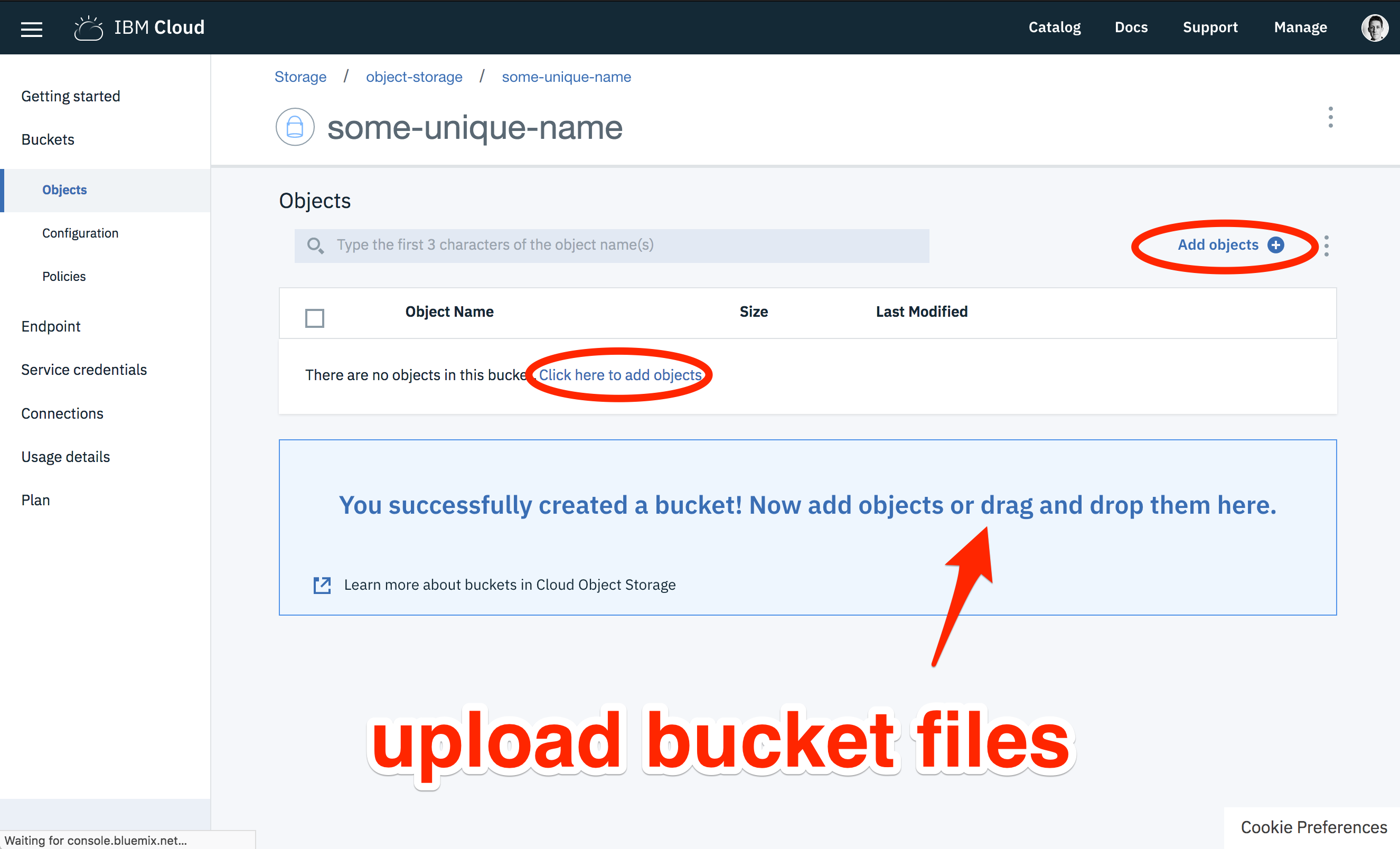
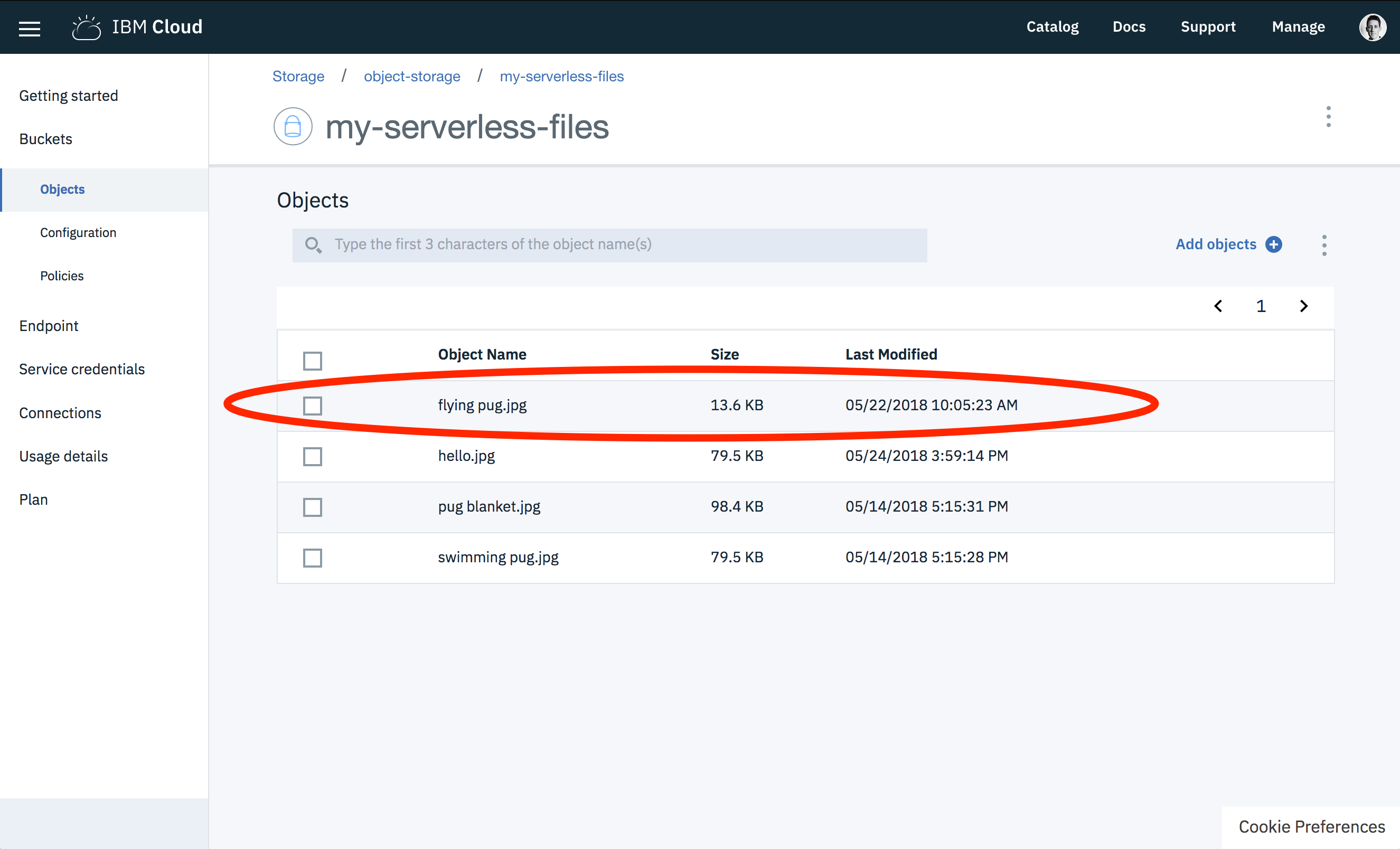

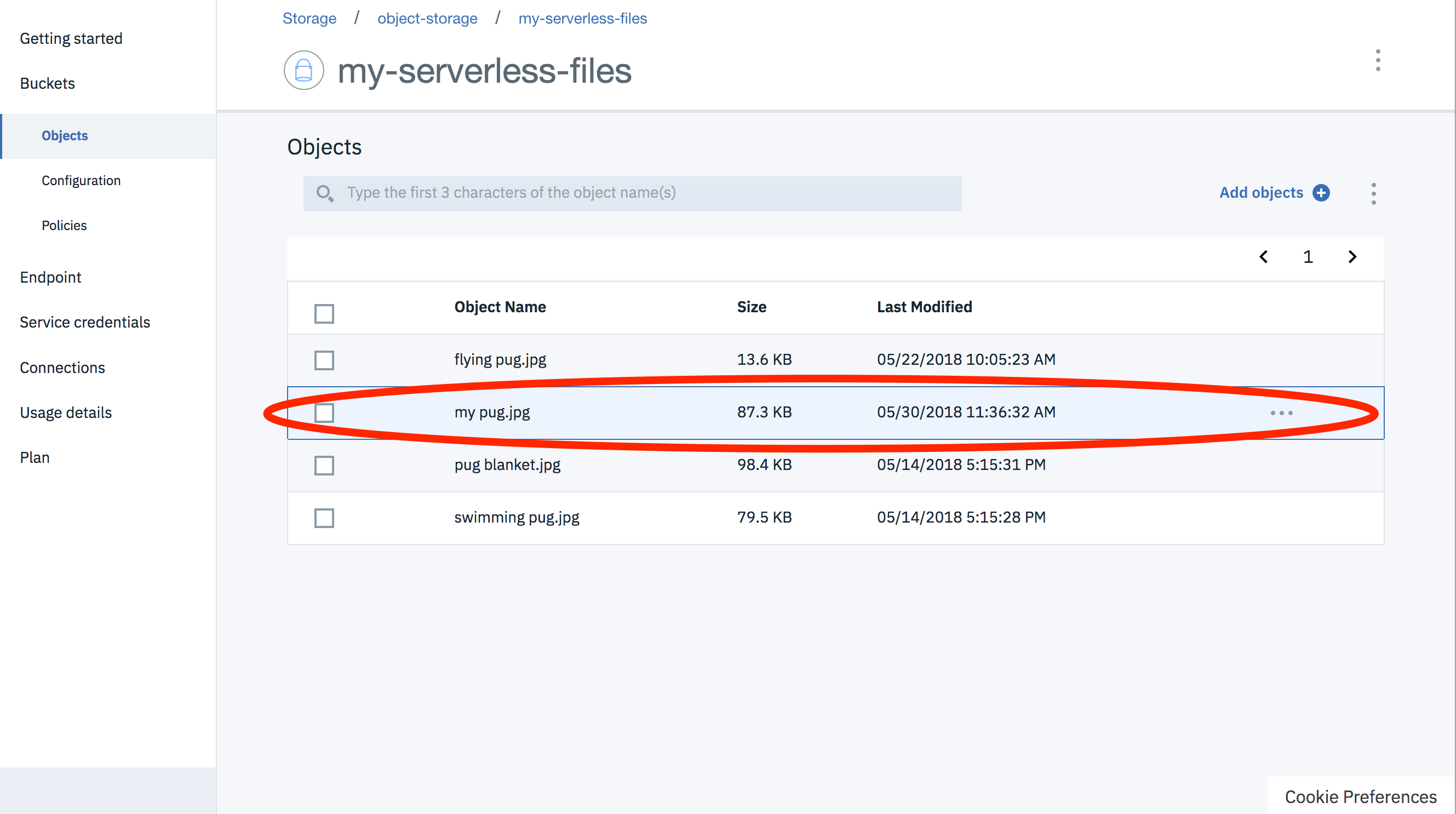
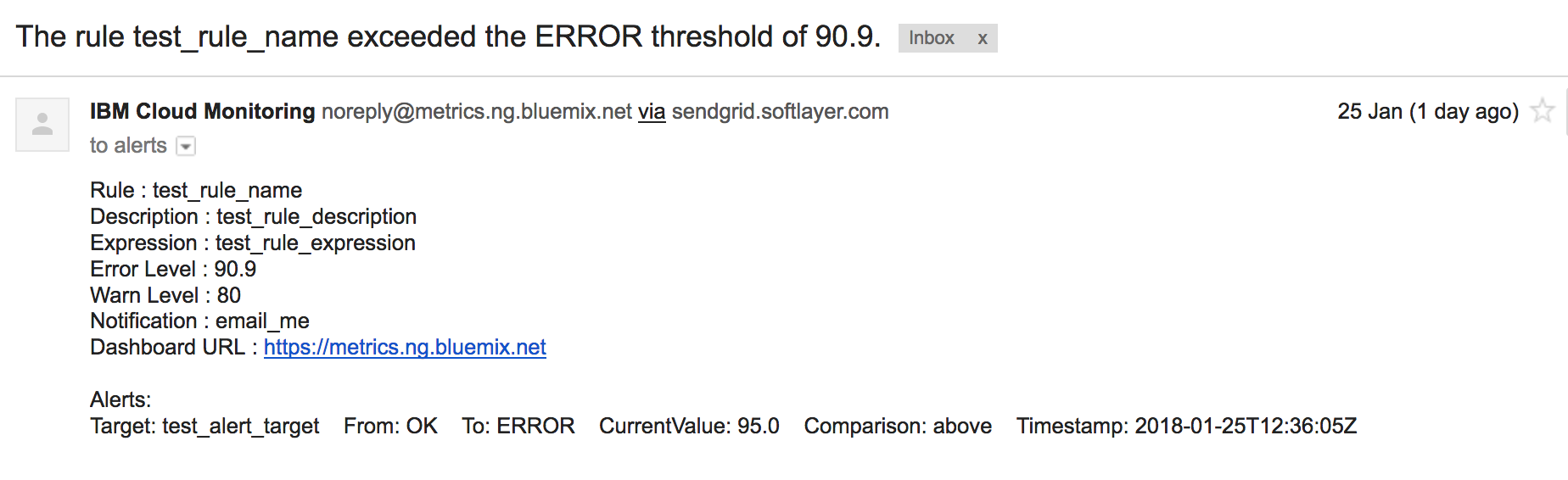

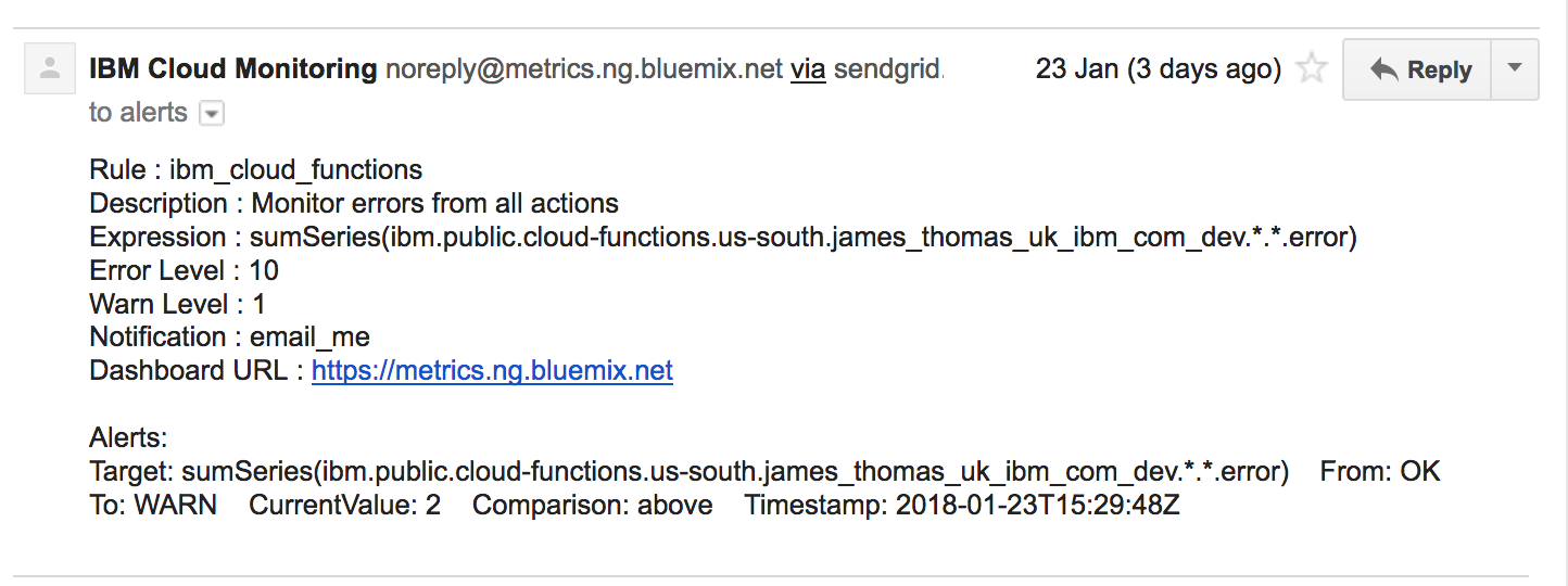


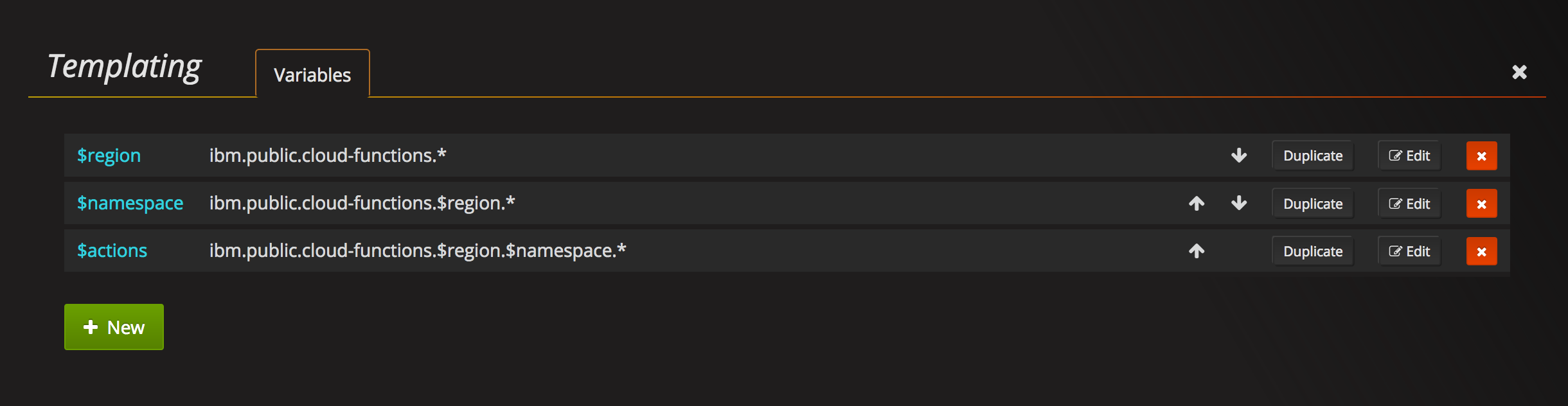
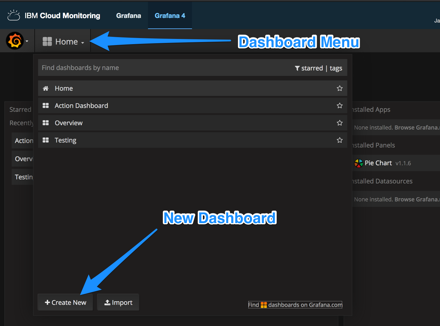
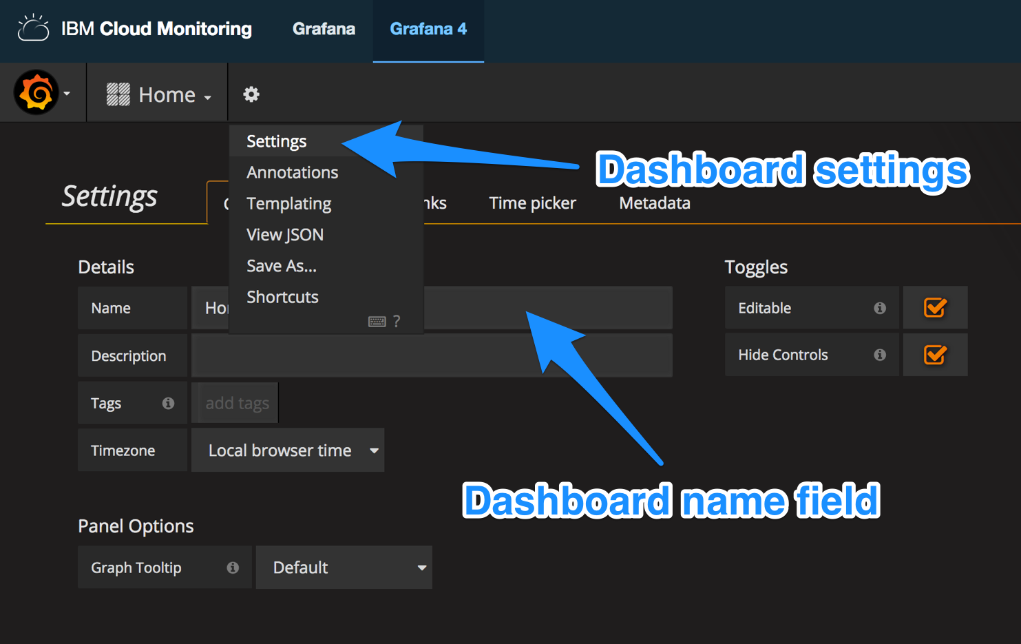
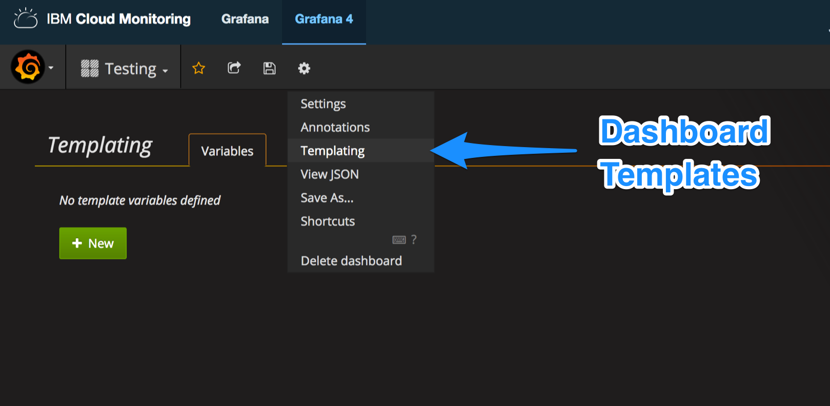
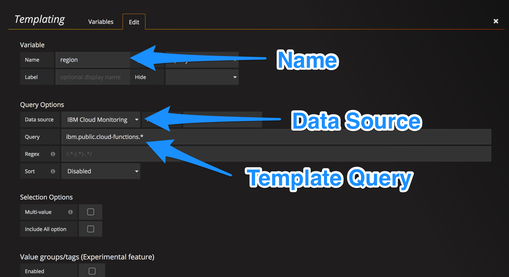
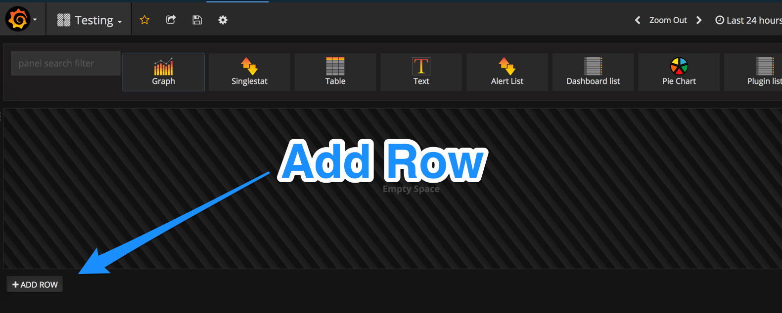
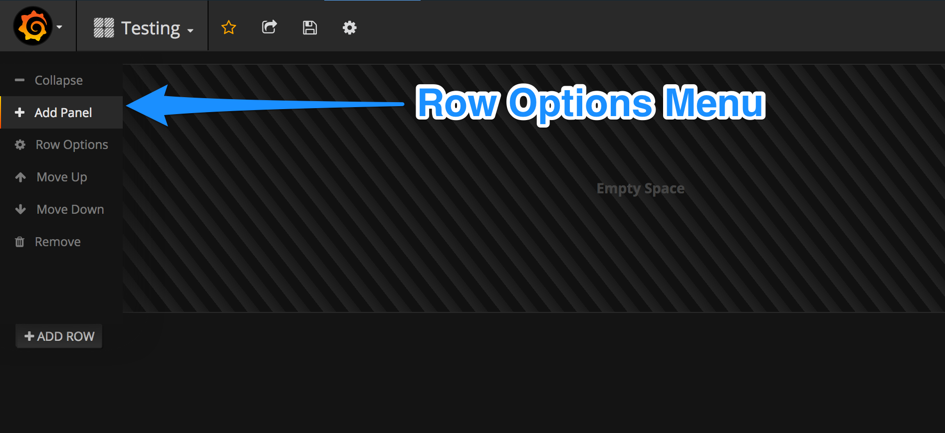
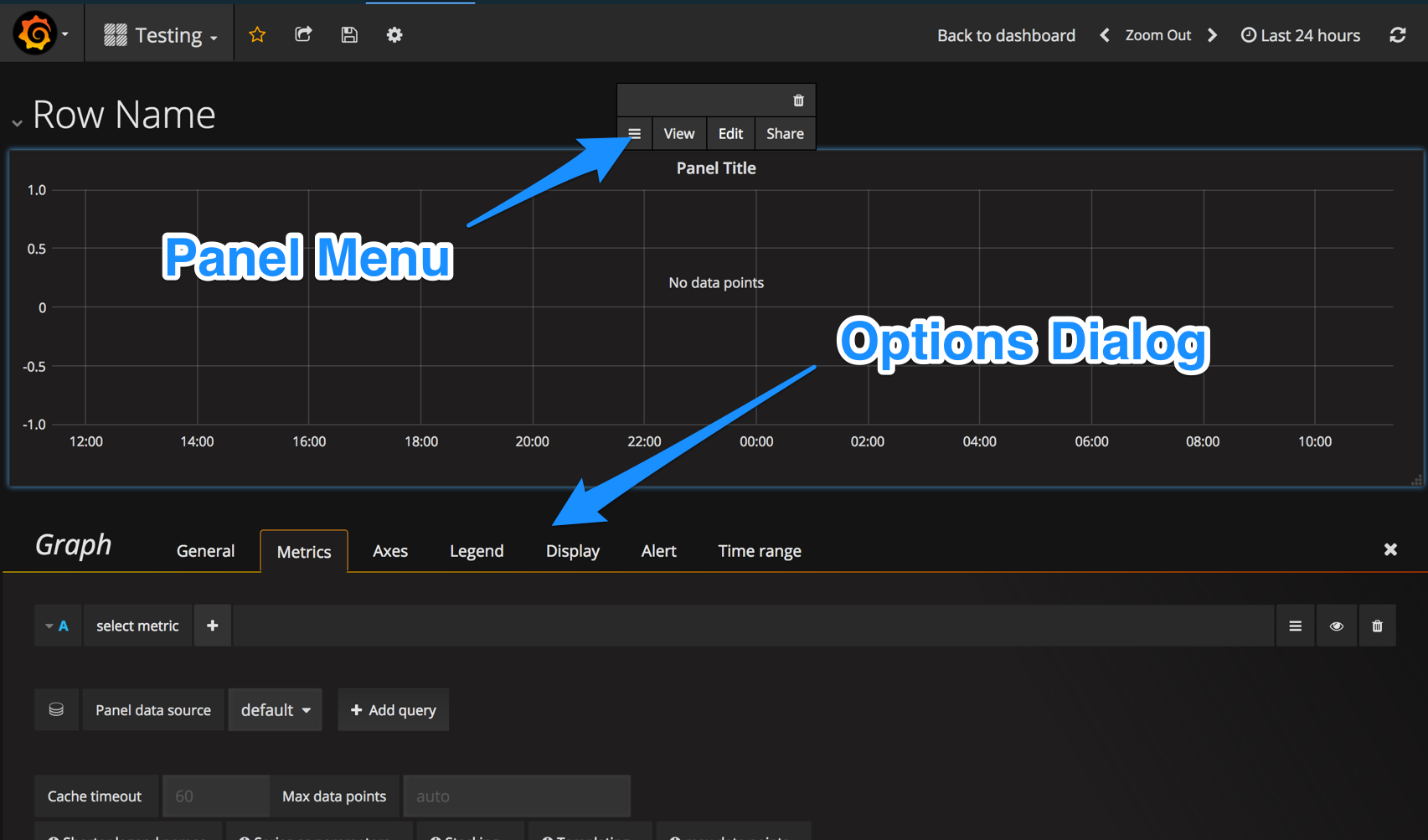
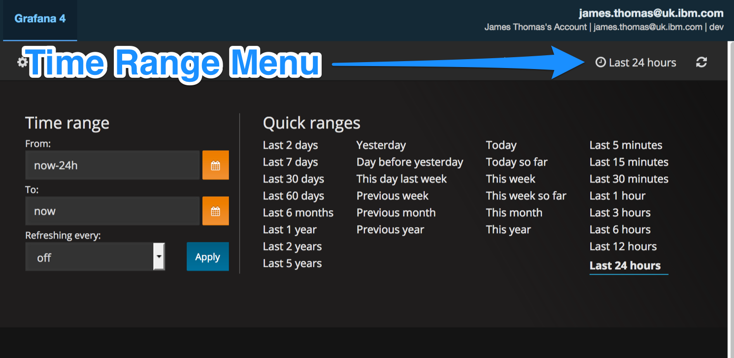
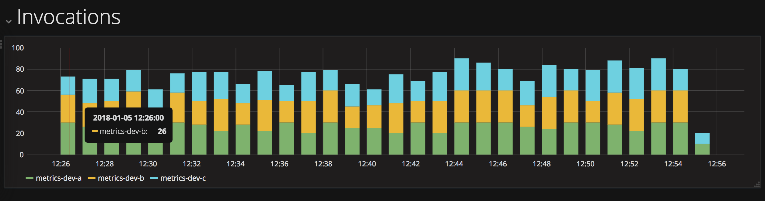
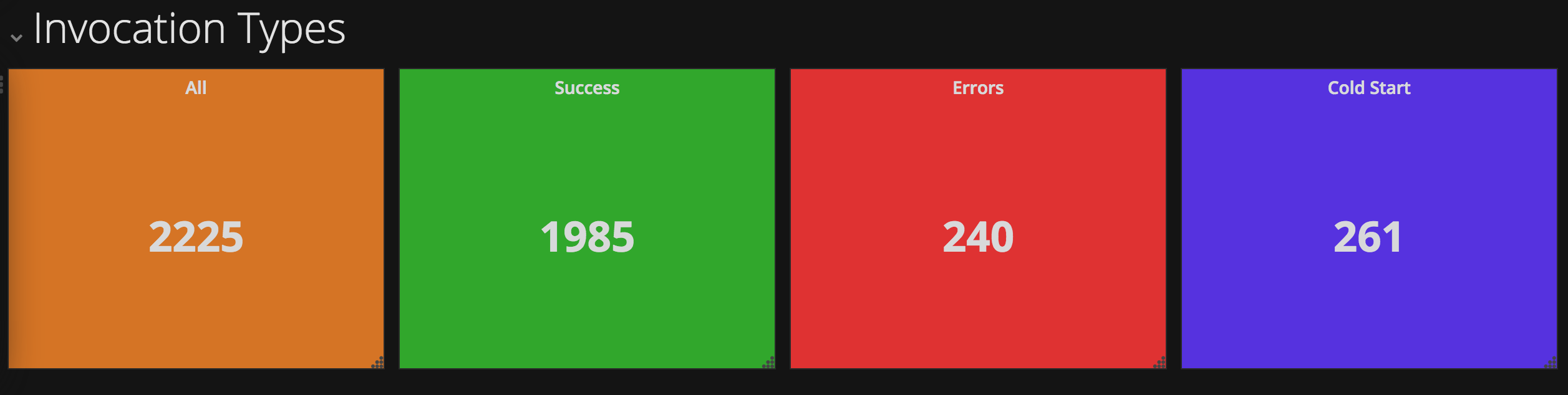
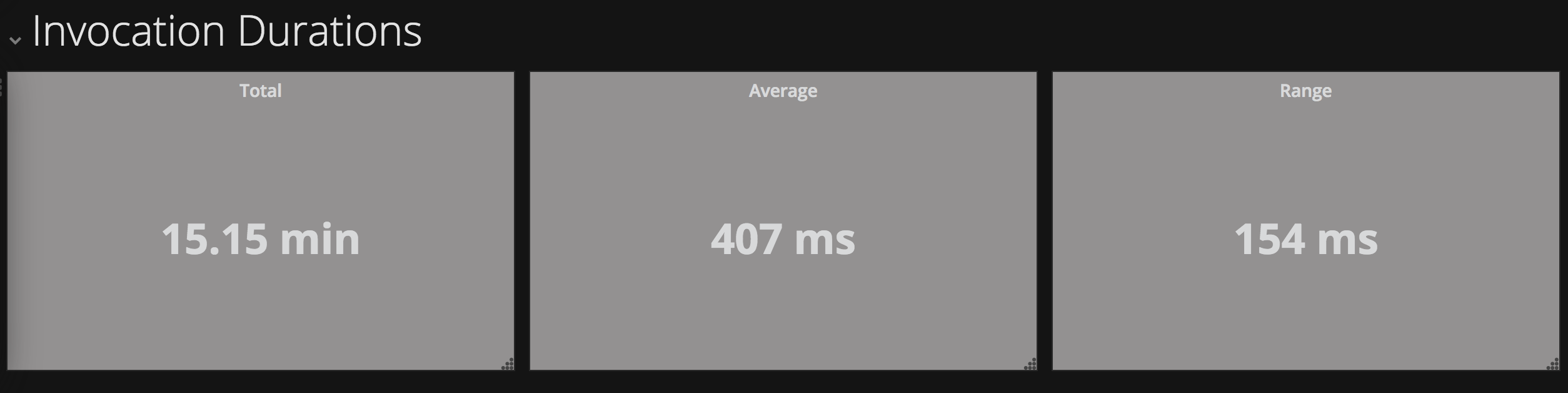
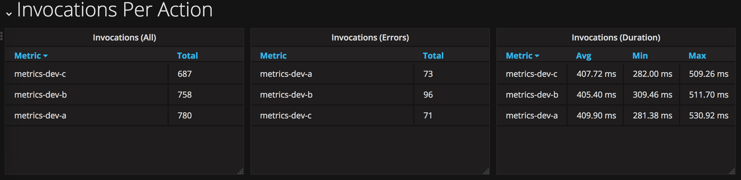
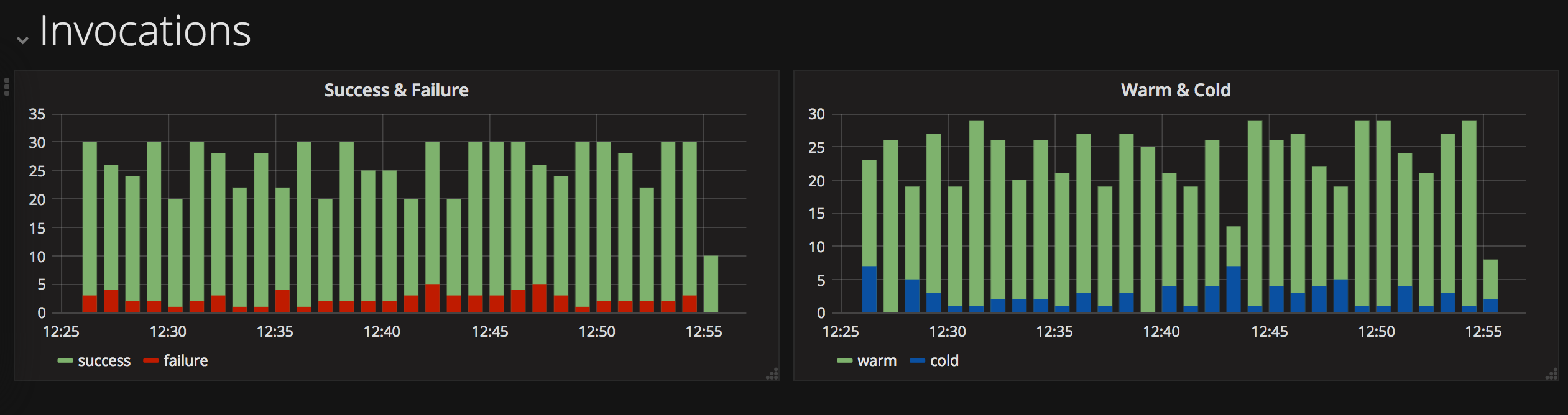
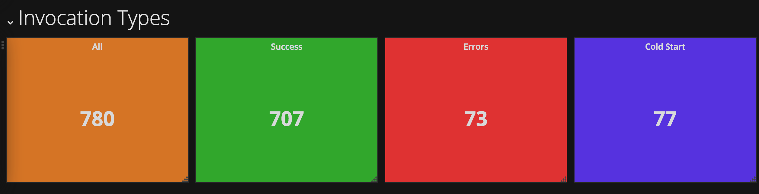
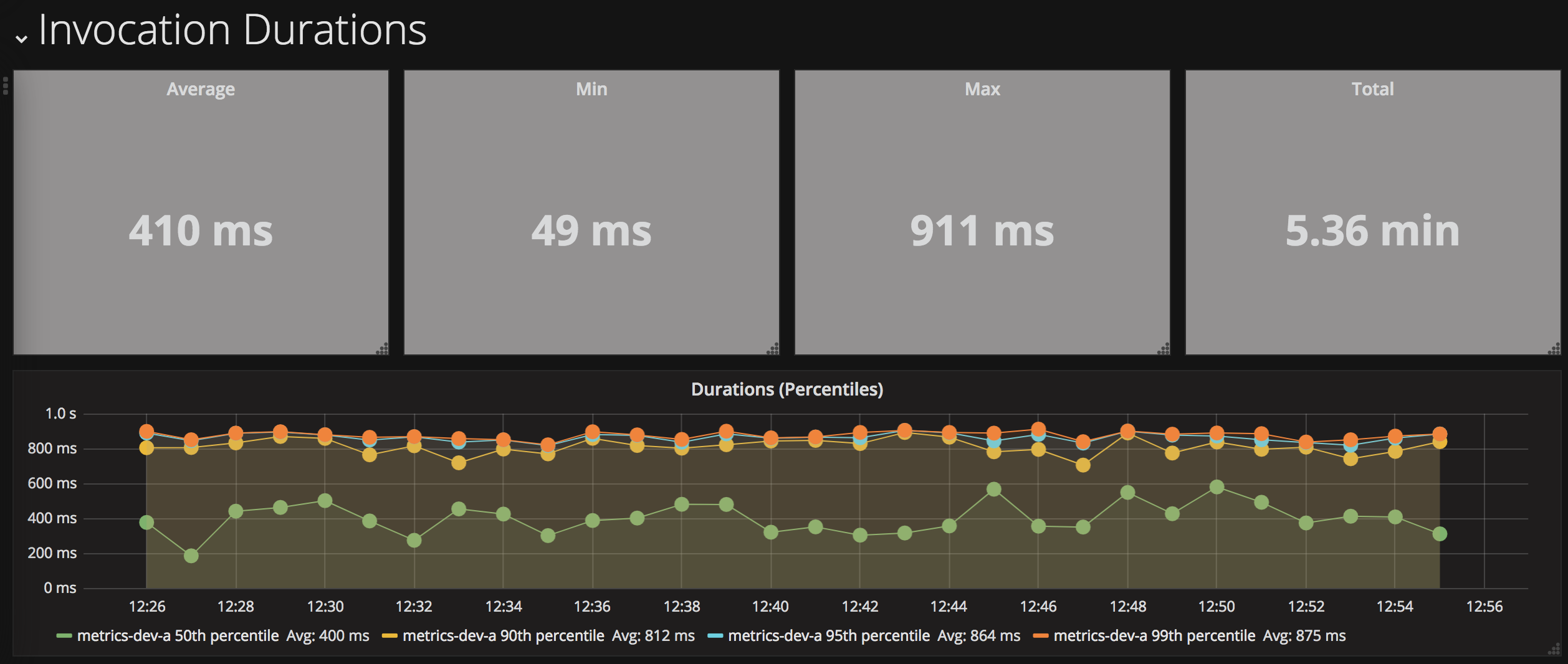
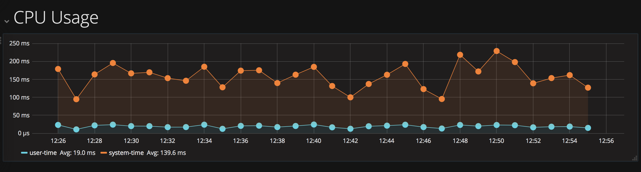
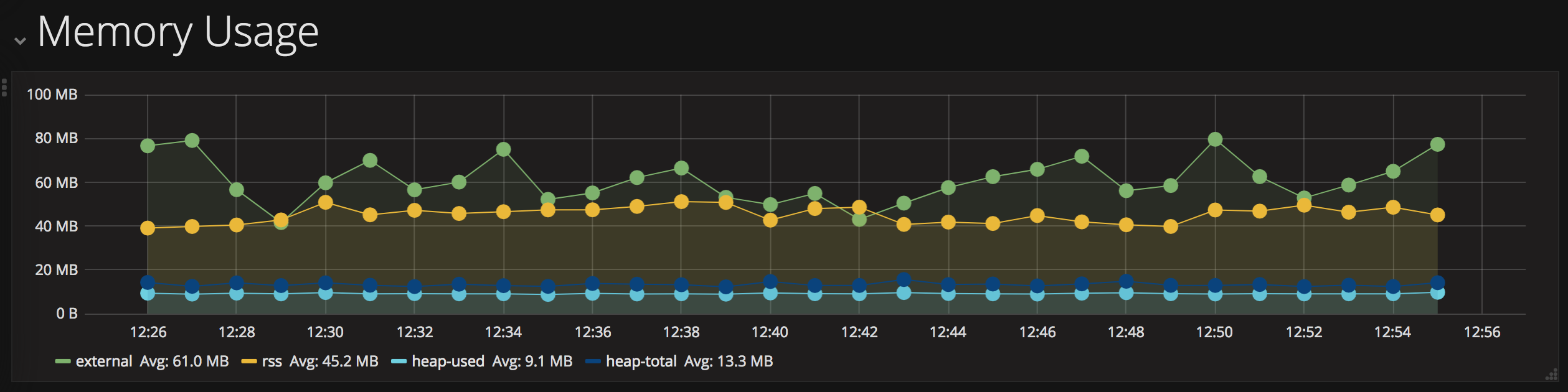